Ask a computer for the value of \((1-\cos x)/x^2\) at \(x=10^{-8}\) . Since \(1-\cos x=\tfrac12x^2-\tfrac1{24}x^4+\cdots\) , the true value is \(0.5\) to fifteen digits. Standard double-precision arithmetic returns exactly \(0\) . Nothing malfunctioned. Every individual operation was carried out as accurately as the machine permits, each with a relative error of about \(10^{-16}\) , and the final answer is wrong in its first digit.
Now ask for \(\ln x\) at \(x=1.0001\) , where \(x\) itself is known only to eight significant digits. However carefully the logarithm is evaluated, the answer can be trusted to about four digits. Here too something was lost, but for a different reason, and no cleverness in the algorithm can recover it.
These two failures are the two halves of this chapter. The first is a defect of an algorithm: a different formula for the same quantity gives all sixteen digits. The second is a property of the problem: the logarithm near \(1\) magnifies relative uncertainty in its input by a factor of ten thousand, and that factor belongs to the mathematics, not to the machine. To tell the two apart one needs a precise model of machine arithmetic, a measure of the sensitivity of a problem, and a way to grade algorithms against that measure. The chapter ends with the first place in the book where two kinds of error pull in opposite directions, the choice of step in a difference quotient.
1.1 Machine numbers and the rounding theorem
A computer stores a real number in a fixed number of digits together with an exponent, as in scientific notation.
Definition 1.1 (floating-point system). Let \(\beta\ge 2\) be an integer base, \(p\ge 1\) an integer precision, and \(e_{\min}\le e_{\max}\) integer exponent bounds. The normalized floating-point system \(\mathbb F(\beta,p,e_{\min},e_{\max})\) consists of \(0\) and all numbers
with \(m\) an integer. Equivalently, each nonzero element is \(\pm\, d_0.d_1d_2\cdots d_{p-1}\times\beta^{e}\) with digits \(0\le d_i\le\beta-1\) and \(d_0\ne 0\) . The elements are called floating-point numbers, or floats. The machine epsilon is \(\varepsilon_{\mathrm{mach}}=\beta^{1-p}\) and the unit roundoff is \(u=\tfrac12\beta^{1-p}\) .
Three features of this set govern everything that follows. It is finite, so there is a largest float and a smallest positive one; results beyond them are said to overflow or underflow. It is not evenly spaced: within one binade \([\beta^{e},\beta^{e+1})\) consecutive floats differ by \(\beta^{e-p+1}\) , so the spacing grows in proportion to the size of the numbers. And relative to that size the spacing is constant: the gap between adjacent floats near \(x\) is roughly \(\varepsilon_{\mathrm{mach}}\lvert x\rvert\) . The machine epsilon is the gap between \(1\) and the next larger float.
The arithmetic used throughout this book is IEEE double precision, the system \(\mathbb F(2,53,-1022,1023)\) . Its machine epsilon is \(2^{-52}\approx 2.22\times10^{-16}\) , its unit roundoff is \(u=2^{-53}\approx 1.11\times10^{-16}\) , its largest float is about \(1.8\times10^{308}\) , and its smallest positive normalized float is \(2^{-1022}\approx 2.2\times10^{-308}\) . The standard adds subnormal numbers below that threshold, signed zeros, infinities, and a not-a-number value; they matter for robust software and play no role in the error analyses of this book, which assume throughout that no overflow or underflow occurs.
For a real number \(x\) within the range of the system, \(\operatorname{fl}(x)\) denotes a float nearest to \(x\) . When \(x\) lies exactly halfway between two floats a rule is needed; IEEE arithmetic picks the neighbour whose last digit is even. The theorem below holds for any tie rule.
Theorem 1.2 (relative error of rounding). Let \(x\) be a real number with \(\beta^{e_{\min}}\le\lvert x\rvert\le x_{\max}\) , where \(x_{\max}\) is the largest float. Then
Proof. By symmetry take \(x>0\) , and let \(e\) be the integer with \(\beta^{e}\le x<\beta^{e+1}\) . The floats in \([\beta^{e},\beta^{e+1}]\) are the multiples \(m\beta^{e-p+1}\) with \(\beta^{p-1}\le m\le\beta^{p}\) , and the hypothesis \(x\le x_{\max}\) guarantees that the two of them bracketing \(x\) belong to the system. They are \(\beta^{e-p+1}\) apart, so the nearer one is within half that distance:
Dividing by \(x\ge\beta^{e}\) gives \(\lvert\operatorname{fl}(x)-x\rvert/x\le\tfrac12\beta^{1-p}=u\) .
The theorem says that storing a number costs a relative error of at most \(u\) , wherever in the enormous range of the system the number lies. That uniformity is the whole point of floating-point representation, and it is why error analysis in this subject is carried out in relative terms.
Example 1.1: Rounding in a three-digit decimal system and in double precision
Take the toy system with \(\beta=10\) and \(p=3\) . Its floats between \(1\) and \(10\) are \(1.00,1.01,\dots,9.99\) , spaced \(0.01\) apart; between \(10\) and \(100\) the spacing is \(0.1\) . The machine epsilon is \(10^{-2}\) and the unit roundoff is \(u=0.005\) .
Rounding \(2/3=0.66666\ldots\) gives \(\operatorname{fl}(2/3)=0.667\) , with relative error \((0.667-0.666\,66\ldots)/0.666\,66\ldots=5.0\times10^{-4}\) . Rounding \(\pi\) gives \(3.14\) , with relative error \(5.07\times10^{-4}\) . Both are well inside the bound \(u=5\times10^{-3}\) of Theorem 1.2. Multiplying the two stored numbers gives \(0.667\times3.14=2.09438\) , which must itself be rounded to three digits: the machine product is \(2.09\) . The true value of \(2\pi/3\) is \(2.094395\ldots\) , so the relative error of the final result is \(2.10\times10^{-3}\) . Three roundings occurred, two on input and one after the multiplication, and the accumulated error is below \(3u\) .
Double precision behaves the same way with \(u=2^{-53}\) . The decimal fraction \(0.1\) is not a binary float, because its binary expansion \(0.000110011001100\ldots\) does not terminate. The stored value is
whose relative error is \(5.55\times10^{-17}\) , exactly \(u/2\) . Consequently the machine sum of the stored values of \(0.1\) and \(0.2\) is the float \(0.3000000000000000444\ldots\) , while the float nearest to \(0.3\) is \(0.2999999999999999889\ldots\) ; they are adjacent floats, \(2^{-54}\approx5.55\times10^{-17}\) apart. A program that tests whether \(0.1+0.2\) equals \(0.3\) receives the answer no. Each number involved is correct to sixteen digits. They are simply not the same float.
1.2 Arithmetic that almost obeys the rules
The exact sum, product, or quotient of two floats is usually not a float. The IEEE standard requires that each of the four basic operations and the square root return the float nearest to the exact result. With Theorem 1.2 this yields the model on which all rounding-error analysis rests.
Definition 1.3 (standard model of floating-point arithmetic). For floats \(x\) and \(y\) and each operation \(\circ\) among \(+\) , \(-\) , \(\times\) , \(/\) , the computed result satisfies
provided no overflow or underflow occurs. The same holds for \(\operatorname{fl}(\sqrt x)\) .
Each operation is therefore as good as it could be. What fails are the laws that connect operations. Floating-point addition is commutative but not associative: in double precision
because floats near \(10^{16}\) are spaced \(2\) apart and \(1+10^{16}\) rounds back to \(10^{16}\) . The distributive law fails similarly. An algorithm is a particular order of operations, and two orders that are algebraically identical can produce different numbers.
How fast can the individual errors build up? A computation with \(n\) operations produces factors \((1+\delta_1)\cdots(1+\delta_n)\) , and the following lemma disposes of such products once and for all.
Lemma 1.4 (accumulated rounding factors). Let \(\lvert\delta_i\rvert\le u\) for \(i=1,\dots,n\) and suppose \(nu<1\) . Then
Proof. Expanding the product and applying the triangle inequality term by term gives \(\lvert\prod(1+\delta_i)-1\rvert\le(1+u)^n-1\) . Since \(1+u\le e^{u}\) , we have \((1+u)^n\le e^{nu}\) , and \(e^{t}\le 1/(1-t)\) for \(0\le t<1\) because \((1-t)e^{t}\) equals \(1\) at \(t=0\) and has derivative \(-te^{t}\le 0\) . Hence \((1+u)^n-1\le 1/(1-nu)-1=nu/(1-nu)\) .
For any \(n\) met in practice \(\gamma_n\) is indistinguishable from \(nu\) : a million operations in double precision give \(\gamma_n\approx10^{-10}\) . Rounding errors accumulate at worst linearly in the number of operations, and that is seldom what ruins a computation. The next result shows the lemma at work and exposes what does.
Proposition 1.5 (recursive summation). Let \(x_1,\dots,x_n\) be floats and let \(\hat s\) be the result of adding them from left to right in floating-point arithmetic. Then \(\hat s=\sum_{i=1}^{n}x_i(1+\theta^{(i)})\) with every \(\lvert\theta^{(i)}\rvert\le\gamma_{n-1}\) , and therefore
Proof. By Definition 1.3 the partial sums satisfy \(\hat s_2=(x_1+x_2)(1+\delta_1)\) and \(\hat s_k=(\hat s_{k-1}+x_k)(1+\delta_{k-1})\) for \(k\ge3\) . Unrolling the recursion, \(x_1\) and \(x_2\) are each multiplied by \((1+\delta_1)\cdots(1+\delta_{n-1})\) , and \(x_i\) for \(i\ge3\) by \((1+\delta_{i-1})\cdots(1+\delta_{n-1})\) . Each product has at most \(n-1\) factors, so Lemma 1.4 gives \(\lvert\theta^{(i)}\rvert\le\gamma_{n-1}\) . Then \(\lvert\hat s-s\rvert=\lvert\sum x_i\theta^{(i)}\rvert\le\gamma_{n-1}\sum\lvert x_i\rvert\) .
The first factor in the bound is tiny. The second, \(\sum\lvert x_i\rvert/\lvert\sum x_i\rvert\) , equals \(1\) when all terms have one sign and is enormous when large terms of opposite sign nearly cancel. Summation is harmless or disastrous according to that ratio, and the ratio is a property of the numbers being summed.
Example 1.2: Ten tenths do not make one
Add the double-precision value of \(0.1\) to itself ten times, starting from \(0\) and accumulating from left to right. The result is
that is, \(1-2^{-53}\) , the float just below \(1\) . The exact sum of the ten stored values is \(10\operatorname{fl}(0.1)=1+5.55\times10^{-17}\) , so the summation error is \(1.67\times10^{-16}\) . Proposition 1.5 with \(n=10\) and all terms positive bounds the relative error by \(\gamma_9\approx9u=1.0\times10^{-15}\) ; the observed error is six times smaller than the bound, which is typical, because the nine rounding errors do not all push the same way.
The lesson for programs is concrete. A loop that advances a time variable by \(0.1\) and stops when the variable equals \(1\) never stops. Compare floats with a tolerance, or count steps with an integer.
1.3 Cancellation
Subtracting two nearly equal numbers is the operation that turns small relative errors into large ones.
Proposition 1.6 (subtraction magnifies relative error). Let \(x\ne y\) be real numbers and let \(\hat x=x(1+\epsilon_x)\) and \(\hat y=y(1+\epsilon_y)\) with \(\lvert\epsilon_x\rvert,\lvert\epsilon_y\rvert\le\epsilon\) . Then
and the bound is attained when \(\epsilon_x=\epsilon\) and \(\epsilon_y=-\epsilon\) with \(x,y>0\) .
Proof. \((\hat x-\hat y)-(x-y)=x\epsilon_x-y\epsilon_y\) , whose absolute value is at most \(\epsilon(\lvert x\rvert+\lvert y\rvert)\) , with equality in the stated case.
Notice what the proposition does not say. It does not say the subtraction is performed inaccurately; by Definition 1.3 the machine subtraction of two floats has relative error at most \(u\) , and when the operands are within a factor of two of each other it is exact (Exercise 1.3). The subtraction is innocent. It exposes errors that the operands already carried. If \(x\) and \(y\) agree in their first \(k\) digits, those digits cancel, the difference has \(k\) fewer significant digits than the operands, and the errors that were in the sixteenth place of \(x\) and \(y\) now sit in the \((16-k)\) -th place of the result. This is catastrophic cancellation.
Example 1.3: The small root of a quadratic
The equation \(x^2-10^{8}x+1=0\) has roots \(x_\pm=\tfrac12\bigl(10^{8}\pm\sqrt{10^{16}-4}\bigr)\) . The larger is very nearly \(10^{8}\) and, because the product of the roots is \(1\) , the smaller is very nearly \(10^{-8}\) ; more precisely \(x_-=1.0000000000000001\times10^{-8}\) .
Evaluate the textbook formula for \(x_-\) in double precision. The number \(10^{16}-4\) is a float. Its square root is \(99\,999\,999.999\,999\,98\) , and the nearest float to that is
since floats near \(10^{8}\) are spaced \(1.49\times10^{-8}\) apart. The relative error of \(d\) is below \(u\) ; it is as good a square root as the machine can hold. Then \(10^{8}-d=1.4901161193847656\times10^{-8}\) , computed exactly, and halving gives
The relative error is \(25\) percent. The eight leading digits of \(10^{8}\) and \(d\) cancelled, and the rounding error in the sixteenth digit of \(d\) was promoted to the first digit of the difference. In the notation of Proposition 1.6, \((\lvert x\rvert+\lvert y\rvert)/\lvert x-y\rvert\approx2\times10^{8}/(2\times10^{-8})=10^{16}\) , which is \(1/u\) .
The repair is to avoid the subtraction. The larger root involves an addition of positive numbers, \(\hat x_+=\tfrac12(10^{8}+d)=10^{8}\) to full accuracy, and the relation \(x_+x_-=1\) then gives
with relative error below \(10^{-16}\) . The general rule for \(ax^2+bx+c=0\) is to compute first the root in which \(-b\) and the signed square root have the same sign, and to obtain the other from the product of the roots \(c/a\) .
The opening puzzle of the chapter is the same phenomenon. At \(x=1.2\times10^{-5}\) the machine holds \(\cos x\) correctly to sixteen digits, and subtracting that float from \(1\) yields \(7.199996\times10^{-11}\) where the true value of \(1-\cos x\) is \(7.1999999999\times10^{-11}\) : the quotient \((1-\cos x)/x^2\) comes out as \(0.49999973\) , with only six correct digits. The identity \(1-\cos x=2\sin^2(x/2)\) involves no subtraction and gives \(0.499999999994\) , correct to every digit shown. At \(x=10^{-8}\) the cosine rounds to exactly \(1\) and the subtractive formula returns \(0\) .
Common mistake. Believing that double precision delivers sixteen correct digits. It delivers sixteen digits per operation. How many survive to the end depends on the sequence of operations, and a single subtraction of nearly equal quantities can remove all of them. The number of digits lost is about \(\log_{10}\bigl((\lvert x\rvert+\lvert y\rvert)/\lvert x-y\rvert\bigr)\) . Before trusting a formula, look for differences of nearly equal quantities and ask whether an algebraic identity, a conjugate, or a series removes them.
1.4 Conditioning: the sensitivity of the problem
Set the machine aside for a moment. Suppose the input \(x\) of a function \(f\) is perturbed slightly. How much does the output move, measured relative to its own size?
Definition 1.7 (relative condition number). Let \(f\) be a real function defined near \(x\) , with \(x\ne0\) and \(f(x)\ne0\) . The relative condition number of \(f\) at \(x\) is
The problem of evaluating \(f\) at \(x\) is well conditioned if \(\kappa_f(x)\) is of modest size and ill conditioned if it is large.
Proposition 1.8 (condition number of a differentiable function). If \(f\) is differentiable at \(x\) , with \(x\ne0\) and \(f(x)\ne0\) , then
Proof. By the definition of the derivative, \(f(x+\delta x)-f(x)=f'(x)\,\delta x+r(\delta x)\) with \(r(\delta x)/\delta x\to0\) as \(\delta x\to0\) . Dividing by \(f(x)\) and by \(\delta x/x\) , the quotient in Definition 1.7 equals \(\lvert x f'(x)/f(x)+x\,r(\delta x)/(f(x)\,\delta x)\rvert\) , and the second term tends to zero uniformly over \(0<\lvert\delta x\rvert\le\epsilon\lvert x\rvert\) as \(\epsilon\to0\) .
The formula makes a table of sensitivities easy to compile. For \(f(x)=\sqrt x\) the condition number is \(\tfrac12\) : square roots halve relative errors. For \(f(x)=x^{\alpha}\) it is \(\lvert\alpha\rvert\) . For \(f(x)=e^{x}\) it is \(\lvert x\rvert\) , so the exponential is sensitive for large arguments. For \(f(x)=x-a\) it is \(\lvert x/(x-a)\rvert\) , which is the content of Proposition 1.6 in one variable: subtraction is ill conditioned when the result is small compared with the operands. And for \(f(x)=\ln x\) it is \(1/\lvert\ln x\rvert\) , which is unbounded as \(x\to1\) .
The meaning of the number is a rule of thumb for digits: if the input is known to a relative accuracy \(\epsilon\) , the output is determined only to a relative accuracy of about \(\kappa\,\epsilon\) , so roughly \(\log_{10}\kappa\) digits are lost. This holds for every algorithm, including a perfect one, because the uncertainty is in the data.
Example 1.4: The logarithm near one
Let \(f(x)=\ln x\) and \(x=1.0001\) . By Proposition 1.8,
Test the prediction directly. Perturb the input by a relative amount \(10^{-8}\) , to \(x(1+10^{-8})\) . The logarithm changes from \(9.99950003\times10^{-5}\) by a relative amount \(1.00005\times10^{-4}\) . The ratio of relative output change to relative input change is \(10000.5\) , as predicted. An input good to eight digits yields a logarithm good to four.
This has a practical consequence for software design. A program that forms \(1+t\) for small \(t\) and then takes the logarithm has already committed a relative rounding error of up to \(u\) in \(1+t\) , and the logarithm magnifies it by \(1/\lvert\ln(1+t)\rvert\approx1/\lvert t\rvert\) . Numerical libraries therefore provide a separate function for \(\ln(1+t)\) that takes \(t\) itself as its argument. As a function of \(t\) , the map \(t\mapsto\ln(1+t)\) has condition number \(\lvert t/((1+t)\ln(1+t))\rvert\approx1\) for small \(t\) . The same quantity is ill conditioned as a function of \(x=1+t\) and well conditioned as a function of \(t\) : conditioning is a property of a problem together with a choice of what counts as its data.
1.5 Stability: the quality of the algorithm
Conditioning grades problems. To grade algorithms we compare what an algorithm actually computes with the exact answer, and there are two ways to measure the discrepancy.
Definition 1.9 (forward error, backward error, backward stability). Let \(\hat y\) be the value an algorithm returns for \(f(x)\) . The forward error is \(\lvert\hat y-f(x)\rvert\) . A backward error is \(\lvert\delta x\rvert\) for a perturbation \(\delta x\) of smallest size such that \(\hat y=f(x+\delta x)\) exactly. The algorithm is backward stable if, for every admissible input, the relative backward error \(\lvert\delta x\rvert/\lvert x\rvert\) is bounded by a modest multiple of the unit roundoff \(u\) .
A backward stable algorithm gives the exact answer to a problem within rounding distance of the one posed. Since the data were rounded on input anyway, that is all one can reasonably ask of an algorithm. Combining the two definitions gives the working principle of the subject.
Proposition 1.10 (forward error from backward error). If \(f\) is differentiable at \(x\) and \(\hat y=f(x+\delta x)\) , then to first order in \(\delta x\) ,
In words: relative forward error is at most about condition number times relative backward error.
Proof. \(\hat y-f(x)=f(x+\delta x)-f(x)=f'(x)\,\delta x+o(\lvert\delta x\rvert)\) . Divide by \(f(x)\) and insert the factor \(x/x\) to obtain \(\bigl(x f'(x)/f(x)\bigr)(\delta x/x)\) plus a term of smaller order.
So a backward stable algorithm applied to a well-conditioned problem gives an accurate answer; applied to an ill-conditioned problem it gives an answer as accurate as the data warrant, and no algorithm can do better. An algorithm is unstable when it produces a large forward error on a well-conditioned problem. That is exactly what the subtractive formula for \(1-\cos x\) does. The function \(x\mapsto1-\cos x\) has condition number \(\lvert x\sin x/(1-\cos x)\rvert\approx2\) for small \(x\) : it is a perfectly well-conditioned problem. The algorithm that first rounds \(\cos x\) to a float and then subtracts is unstable, because the rounding error in \(\cos x\) , harmless in itself, is not the effect of any small relative change in \(x\) . The half-angle formula is a stable algorithm for the same problem. In Example 1.4, by contrast, no reformulation in terms of \(x\) helps, because the problem itself is ill conditioned.
Instability is not always a matter of one bad subtraction. It can be spread over many steps, each of which looks harmless.
Example 1.5: A recurrence that destroys its own answer
Let \(I_n=\int_0^1x^{n}e^{x-1}\,dx\) for \(n\ge0\) . Integration by parts gives
On \([0,1]\) the integrand lies between \(0\) and \(x^{n}\) , so \(0<I_n<1/(n+1)\) : the values decrease slowly to zero. Running the recurrence forward in double precision gives \(\hat I_{10}=0.0838770701\) , correct in every digit shown, then
The true values are \(I_{15}=0.059018\) , \(I_{18}=0.050120\) , and \(I_{20}=0.045545\) . A negative value for the integral of a positive function is a certain sign of trouble.
The cause is visible in the recurrence. If \(\hat I_{n-1}=I_{n-1}+e_{n-1}\) , then \(\hat I_n=I_n-n\,e_{n-1}\) : each step multiplies the inherited error by \(-n\) . After \(n\) steps the initial error has been multiplied by \(n!\) in magnitude. The stored value of \(I_0\) differs from \(1-e^{-1}\) by \(1.24\times10^{-17}\) , and \(20!\approx2.43\times10^{18}\) ; the product is \(30.2\) , which accounts for the computed \(\hat I_{20}\) almost exactly. Every step is a single multiplication and a single subtraction, each performed to full machine accuracy.
Run the same relation backward, as \(I_{n-1}=(1-I_n)/n\) . Now each step divides the inherited error by \(n\) . Start from the crude guess \(I_{30}\approx0\) , whose error is less than \(1/31\) . After ten backward steps the error has been divided by \(30\cdot29\cdots21\approx1.1\times10^{14}\) , and the computed value
agrees with the true \(I_{20}=0.045544884075818\ldots\) to fifteen digits. Continuing down to \(n=0\) reproduces \(I_0\) to the last digit. The forward recurrence is an unstable algorithm and the backward recurrence is a stable one, for the same sequence of numbers.
Common mistake. Describing a wrong answer as “caused by an ill-conditioned problem” without computing a condition number, or blaming “rounding error” in general. The diagnosis has two separate parts. Compute or estimate \(\kappa\) for the problem as posed. If \(\kappa u\) already accounts for the observed error, the problem is ill conditioned and only better data or a reformulated problem will help. If \(\kappa\) is modest and the error is large, the algorithm is unstable and should be replaced. In Example 1.5 the integrals \(I_n\) are tame functions of \(n\) ; only the forward route to them is unstable.
1.6 When truncation meets rounding
Most numerical methods replace a limit by a finite expression, and the resulting truncation error shrinks as some parameter \(h\) shrinks. Rounding error usually grows as \(h\) shrinks. The simplest case shows the conflict in full, and the same picture reappears for quadrature and for differential equations in later chapters.
The tool is Taylor’s theorem: if \(f\) has \(n+1\) continuous derivatives on an interval containing \(x\) and \(x+h\) , then
for some \(\xi\) between \(x\) and \(x+h\) . It is proved in Calculus, where it extends the tangent-line approximation to higher order with an explicit remainder, and it will be used in nearly every chapter of this book.
Approximate \(f'(x)\) by the forward difference \(D_hf(x)=\bigl(f(x+h)-f(x)\bigr)/h\) . Suppose the values of \(f\) are not available exactly but only as computed values \(\hat f\) with \(\lvert\hat f(t)-f(t)\rvert\le\epsilon_f\) ; at best \(\epsilon_f\approx u\lvert f(x)\rvert\) .
Theorem 1.11 (error of the forward difference). Let \(f\) be twice continuously differentiable on \([x,x+h]\) with \(\lvert f''\rvert\le M\) there, and let \(\hat D_h=\bigl(\hat f(x+h)-\hat f(x)\bigr)/h\) with \(\lvert\hat f-f\rvert\le\epsilon_f\) . Then
The right side is smallest at \(h^\star=2\sqrt{\epsilon_f/M}\) , where it equals \(2\sqrt{M\epsilon_f}\) .
Proof. Taylor’s theorem with \(n=1\) gives \(f(x+h)=f(x)+hf'(x)+\tfrac12h^2f''(\xi)\) , so \(\lvert D_hf(x)-f'(x)\rvert=\tfrac12h\lvert f''(\xi)\rvert\le Mh/2\) . The perturbed quotient differs from the exact one by \(\bigl((\hat f-f)(x+h)-(\hat f-f)(x)\bigr)/h\) , which is at most \(2\epsilon_f/h\) in absolute value. The triangle inequality gives the bound. Its derivative with respect to \(h\) is \(M/2-2\epsilon_f/h^2\) , which vanishes at \(h^\star\) , and substituting gives \(M h^\star/2+2\epsilon_f/h^\star=2\sqrt{M\epsilon_f}\) .
With \(\epsilon_f\approx u\) the best step is of order \(\sqrt u\approx10^{-8}\) and the best attainable error is also of order \(\sqrt u\) : a forward difference in double precision cannot deliver more than about eight digits of a derivative, whatever \(h\) is used. The symmetric central difference \(\bigl(f(x+h)-f(x-h)\bigr)/(2h)\) has truncation error bounded by \(M_3h^2/6\) , where \(M_3\) bounds \(\lvert f'''\rvert\) , and rounding error bounded by \(\epsilon_f/h\) . Its best step is \((3\epsilon_f/M_3)^{1/3}\) , of order \(u^{1/3}\approx10^{-5}\) , and its best error is of order \(u^{2/3}\approx10^{-11}\) (Exercise 1.11). Higher order buys a larger optimal step and a smaller optimal error, but the rounding term never disappears.
Example 1.6: Differentiating the exponential at one
Let \(f(x)=e^{x}\) and \(x=1\) , so that \(f'(1)=e\) . Both differences were evaluated in double precision for \(h=10^{-1},10^{-2},\dots,10^{-12}\) . The absolute errors are:
| \(h\) | forward difference error | central difference error |
|---|---|---|
| \(10^{-1}\) | \(1.406\times10^{-1}\) | \(4.533\times10^{-3}\) |
| \(10^{-2}\) | \(1.364\times10^{-2}\) | \(4.530\times10^{-5}\) |
| \(10^{-3}\) | \(1.360\times10^{-3}\) | \(4.530\times10^{-7}\) |
| \(10^{-4}\) | \(1.359\times10^{-4}\) | \(4.531\times10^{-9}\) |
| \(10^{-5}\) | \(1.359\times10^{-5}\) | about \(6\times10^{-11}\) |
| \(10^{-6}\) | \(1.359\times10^{-6}\) | about \(2\times10^{-10}\) |
| \(10^{-8}\) | about \(7\times10^{-9}\) | about \(7\times10^{-9}\) |
| \(10^{-10}\) | about \(2\times10^{-6}\) | about \(7\times10^{-7}\) |
| \(10^{-12}\) | about \(4\times10^{-4}\) | about \(2\times10^{-4}\) |
In the upper rows the forward error is \(1.359\,h\) , which is \(\tfrac12f''(1)h=\tfrac12eh\) , and the central error is \(0.4530\,h^2\) , which is \(\tfrac16f'''(1)h^2=\tfrac16eh^2\) : truncation dominates and each error follows its Taylor prediction to four digits. In the lower rows the errors grow like \(1/h\) and their leading digits are rounding noise; on a different machine or with a different exponential routine those entries change, though not their order of magnitude. For this function \(M\approx e\) and \(\epsilon_f\approx ue=3.0\times10^{-16}\) , so Theorem 1.11 predicts a best forward step \(h^\star=2\sqrt u=2.1\times10^{-8}\) and a best error bound \(2e\sqrt u=5.7\times10^{-8}\) . The observed error at \(h=10^{-8}\) is below that bound, and the rounding bound \(2\epsilon_f/h=6\times10^{-4}\) at \(h=10^{-12}\) is of the size observed.
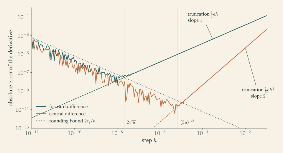
Figure 1.1 is the picture to remember. On logarithmic axes a truncation error proportional to \(h^{p}\) is a straight line of slope \(p\) , and a rounding error proportional to \(u/h\) is a straight line of slope \(-1\) . The measured error follows whichever is larger. To the right of the crossing the curve is smooth and its slope reveals the order of the method; to the left it is ragged, because rounding errors are not smooth functions of \(h\) . Reading the order of a method from the slope of such a plot, and recognising the rounding floor when it appears, is a skill used in every later chapter.
The moral is a habit of mind. A numerical answer comes with three separate questions. How sensitive is the problem to its data? How much error did the method introduce by truncating an infinite process? How much did finite-precision arithmetic add, and was it amplified? The remaining chapters answer the second question for one class of methods after another, and return to the first and third whenever they threaten the result.
Exercises
-
In the decimal system with \(\beta=10\) and \(p=4\) , give the unit roundoff, the spacing of the floats between \(100\) and \(1000\) , and \(\operatorname{fl}(1/7)\) and \(\operatorname{fl}(22/7)\) ; compute the relative error of each rounding and confirm that Theorem 1.2 holds.
Answer
The unit roundoff is \(u=\tfrac12\cdot10^{-3}=5\times10^{-4}\) , and floats between \(100\) and \(1000\) are spaced \(0.1\) apart. \(\operatorname{fl}(1/7)=0.1429\) with relative error \(3.0\times10^{-4}\) , and \(\operatorname{fl}(22/7)=3.143\) with relative error \(4.5\times10^{-5}\) . Both are below \(u\) .
-
For IEEE double precision, find the two floats adjacent to \(1\) , explain why the gap above \(1\) is twice the gap below, and determine the smallest positive integer that is not a float.
Answer
The neighbours of \(1\) are \(1-2^{-53}\) and \(1+2^{-52}\) . Just below \(1\) the floats lie in the binade \([\tfrac12,1)\) , where the spacing is \(2^{-53}\) ; from \(1\) upward they lie in \([1,2)\) , where it is \(2^{-52}\) . All integers up to \(2^{53}\) are floats; in \([2^{53},2^{54})\) the spacing is \(2\) , so the first integer that is not a float is \(2^{53}+1=9007199254740993\) .
-
Let \(x\) and \(y\) be floats in a system with base \(\beta\) and precision \(p\) satisfying \(y/2\le x\le 2y\) , and assume no underflow. Prove that \(x-y\) is a float, so that the machine subtraction is exact.
Solution
The hypothesis \(y/2\le x\le2y\) forces \(x\) and \(y\) to have the same sign, and replacing both by their negatives changes nothing, so take \(y>0\) . If \(x<y\) , interchange the roles of \(x\) and \(y\) : the hypothesis is symmetric, because \(y/2\le x\le2y\) is equivalent to \(x/2\le y\le2x\) , and the negative of a float is a float. So assume \(0<y\le x\le2y\) .
Write \(y=m_y\,q\) with \(q=\beta^{e_y-p+1}\) and \(\beta^{p-1}\le m_y\le\beta^{p}-1\) . Since \(x\ge y\) , the exponent of \(x\) is at least \(e_y\) , so the spacing of floats at \(x\) is a multiple of \(q\) by a nonnegative power of \(\beta\) , and \(x\) is an integer multiple of \(q\) . Hence \(x-y=kq\) for an integer \(k\ge0\) . The hypothesis \(x\le2y\) gives \(x-y\le y\) , that is, \(k\le m_y\le\beta^{p}-1\) .
A number \(kq\) with \(0\le k\le\beta^{p}-1\) is a float: if \(k=0\) it is zero, and otherwise \(k\) has at most \(p\) digits in base \(\beta\) , so multiplying \(k\) by a suitable power of \(\beta\) and lowering the exponent by the same amount puts the significand in the normalized range \([\beta^{p-1},\beta^{p}-1]\) . Lowering the exponent is permitted because no underflow occurs. Therefore \(x-y\) is exactly representable, and since the machine subtraction returns the float nearest the exact difference, it returns the exact difference.
-
In the decimal system with \(p=3\) , add the eleven numbers \(1.00,0.004,0.004,\dots,0.004\) from left to right and then from right to left, rounding after every addition; explain the difference using Proposition 1.5 and state a rule for the order in which positive numbers should be summed.
Solution
Left to right. The first addition is \(1.00+0.004=1.004\) , which lies between the adjacent floats \(1.00\) and \(1.01\) and rounds to \(1.00\) . Every later addition repeats this, so the final result is \(1.00\) . The ten small terms have vanished completely.
Right to left. The partial sums of the small terms are \(0.004,0.008,0.012,\dots,0.040\) , each with at most two significant digits and hence a float; no rounding occurs. The last addition \(0.040+1.00\) gives \(1.04\) , which is the exact sum.
Explanation. In the proof of Proposition 1.5 the error committed at step \(k\) is \(\delta_{k-1}\) times the partial sum at that step. When the large term comes first, every partial sum is about \(1\) , so every step may commit an absolute error up to \(u\cdot1=0.005\) , larger than the term being added. When the small terms come first the partial sums stay small while they are being accumulated, and so do the absolute errors. Equivalently, the first term summed is multiplied by \(n-1\) rounding factors and the last by one, so the large terms should enter last. The rule: sum positive numbers in order of increasing magnitude.
-
With \(\beta=10\) , \(p=3\) , \(x=3.34\) , and \(y=3.33\) , compute \(x^2-y^2\) by forming the two squares first and by the product \((x-y)(x+y)\) , rounding after every operation; compare with the exact value and explain the outcome using Proposition 1.6.
Solution
Squares first. \(x^2=11.1556\) rounds to \(11.2\) and \(y^2=11.0889\) rounds to \(11.1\) . Their difference is formed exactly, and the computed difference is \(0.1\) .
Product form. \(x-y=0.01\) and \(x+y=6.67\) are both exact, and \(0.01\times6.67=0.0667\) needs no rounding.
The exact value is \(x^2-y^2=0.0667\) , so the product form is exact and the squares-first form has a relative error of \(50\) percent. In Proposition 1.6 the operands are \(a=x^2\) and \(b=y^2\) , each rounded with relative error at most \(u=0.005\) , and the amplification factor is \((\lvert a\rvert+\lvert b\rvert)/\lvert a-b\rvert=22.24/0.0667\approx333\) . The bound on the relative error of the difference is therefore \(0.005\times333\approx1.7\) , and the observed \(0.5\) lies within it. The squares agree in their leading two digits, those digits cancel, and the rounding errors of the squares, which were in the third digit, become errors in the first digit of the result. The product form subtracts the data \(x\) and \(y\) , which carry no rounding error, so its cancellation is harmless.
-
Rewrite each expression so that it can be evaluated without cancellation in the stated regime, and evaluate \(\sqrt{x+1}-\sqrt{x}\) at \(x=10^{12}\) both ways in double precision: (a) \(\sqrt{x+1}-\sqrt x\) for large \(x\) ; (b) \(\ln(x+1)-\ln x\) for large \(x\) ; (c) \(1/(1+2x)-(1-x)/(1+x)\) for small \(\lvert x\rvert\) .
Answer
(a) \(1/(\sqrt{x+1}+\sqrt x)\) . (b) \(\ln(1+1/x)\) , evaluated with the library function for \(\ln(1+t)\) at \(t=1/x\) . (c) Over a common denominator the numerator is \((1+x)-(1-x)(1+2x)=2x^2\) , so the expression equals \(2x^2/\bigl((1+2x)(1+x)\bigr)\) . At \(x=10^{12}\) the subtractive form of (a) gives \(5.00003807\times10^{-7}\) and the stable form gives \(4.99999999999875\times10^{-7}\) , which is correct to all digits shown: the naive value has five correct digits.
-
Compute the relative condition number of each function and say where it is large: (a) \(\tan x\) near \(\pi/2\) , with a value at \(x=1.57\) ; (b) \(\arcsin x\) near \(1\) , with a value at \(x=0.9999\) ; (c) \(x^{10}\) ; (d) \(x/(1-x)\) .
Answer
(a) \(\kappa=\lvert x/(\sin x\cos x)\rvert=\lvert2x/\sin2x\rvert\) , unbounded as \(x\to\pi/2\) ; at \(x=1.57\) it is about \(1972\) . (b) \(\kappa=x/\bigl(\sqrt{1-x^2}\,\arcsin x\bigr)\) , unbounded as \(x\to1\) ; at \(x=0.9999\) it is about \(45.4\) . (c) \(\kappa=10\) everywhere. (d) \(f'(x)=1/(1-x)^2\) , so \(\kappa=1/\lvert1-x\rvert\) , large near \(x=1\) .
-
Prove that for differentiable \(f\) and \(g\) the condition number of the composition satisfies \(\kappa_{g\circ f}(x)=\kappa_g(f(x))\,\kappa_f(x)\) , and use this with \(f=\cos\) and \(g(c)=1-c\) to explain why evaluating \(1-\cos x\) in two stages is unstable for small \(x\) although the composite problem is well conditioned.
Solution
By the chain rule \((g\circ f)'(x)=g'(f(x))\,f'(x)\) . Proposition 1.8 gives
\[ \kappa_{g\circ f}(x)=\left\lvert\frac{x\,g'(f(x))\,f'(x)}{g(f(x))}\right\rvert =\left\lvert\frac{f(x)\,g'(f(x))}{g(f(x))}\right\rvert\cdot\left\lvert\frac{x\,f'(x)}{f(x)}\right\rvert =\kappa_g(f(x))\,\kappa_f(x), \]where the middle step multiplies and divides by \(f(x)\ne0\) .
Take \(f(x)=\cos x\) and \(g(c)=1-c\) . Then \(\kappa_f(x)=\lvert x\tan x\rvert\approx x^2\) for small \(x\) , and \(\kappa_g(c)=\lvert c/(1-c)\rvert\approx2/x^2\) at \(c=\cos x\) . Their product is about \(2\) : the composite problem is well conditioned. But the two-stage algorithm does not hand the second stage the exact \(f(x)\) ; it hands it \(\operatorname{fl}(\cos x)\) , which carries a relative error up to \(u\) . The second stage is an ill-conditioned problem, and it magnifies that error by \(\kappa_g\approx2/x^2\) . At \(x=1.2\times10^{-5}\) this predicts a relative error up to \(1.4\times10^{10}\,u\approx1.5\times10^{-6}\) , consistent with the observed error of \(5\times10^{-7}\) in Example 1.3. The tiny factor \(\kappa_f\approx x^2\) describes how little \(\cos x\) responds to errors in \(x\) ; it does nothing to shrink an error introduced after the first stage. A well-conditioned problem factored through an ill-conditioned intermediate problem gives an unstable algorithm.
-
A student writes: “Each operation in \((1-\cos x)/x^2\) has relative error at most \(u\) , and there are four operations, so by Lemma 1.4 the result has relative error at most \(\gamma_4\) .” Identify the step in the evaluation to which the standard model was applied incorrectly, and state what a correct bound must contain.
Hint
Lemma 1.4 controls a product of factors \((1+\delta_i)\) . Write out what the machine computes: \(\hat c=\cos x\,(1+\delta_1)\) , then \((1-\hat c)(1+\delta_2)\) . Is \(1-\cos x\,(1+\delta_1)\) equal to \((1-\cos x)\) times a factor close to \(1\) ? A correct bound must contain the amplification factor of Proposition 1.6 for the subtraction, here \((1+\cos x)/(1-\cos x)\approx4/x^2\) .
-
Let \(p_n=\int_0^1x^{n}/(x+5)\,dx\) . Show that \(p_n+5p_{n-1}=1/n\) and \(p_0=\ln(6/5)\) , explain why the forward recurrence loses accuracy and estimate how many digits remain at \(n=20\) , and describe a stable way to compute \(p_{20}\) , including a justified starting value.
Solution
Adding the integrands, \(p_n+5p_{n-1}=\int_0^1x^{n-1}(x+5)/(x+5)\,dx=\int_0^1x^{n-1}\,dx=1/n\) , and \(p_0=\int_0^1dx/(x+5)=\ln6-\ln5\) .
Forward. Solving for \(p_n\) gives \(p_n=1/n-5p_{n-1}\) . An error \(e_{n-1}\) in \(p_{n-1}\) becomes \(-5e_{n-1}\) in \(p_n\) , so after twenty steps the initial rounding error, of size about \(u\,p_0\approx2\times10^{-17}\) , has grown by \(5^{20}\approx9.5\times10^{13}\) to about \(2\times10^{-3}\) , and the rounding errors of the intermediate steps are amplified similarly. Since \(x^{20}/6\le x^{20}/(x+5)\le x^{20}/5\) on \([0,1]\) , the true value satisfies \(1/126\le p_{20}\le1/105\) , so \(p_{20}\approx0.008\) and an absolute error of a few times \(10^{-3}\) leaves no correct digit. Indeed the forward recurrence in double precision returns \(0.0042\) .
Backward. Solving instead for \(p_{n-1}\) gives \(p_{n-1}=(1/n-p_n)/5\) , and now each step divides the inherited error by \(5\) . Start at \(n=40\) with the guess \(p_{40}\approx0\) ; by the same bounds \(0<p_{40}<1/205\) , so the starting error is below \(0.005\) . Twenty backward steps reduce it by \(5^{20}\) to below \(10^{-16}\) , and rounding errors made along the way are damped in the same manner. The result is \(p_{20}=0.00799752302823\) , correct to all digits shown. The forward direction is unstable and the backward direction stable, exactly as in Example 1.5, with the fixed factor \(5\) in place of the growing factor \(n\) .
-
Derive the error bound \(M_3h^2/6+\epsilon_f/h\) for the central difference under the assumptions of Theorem 1.11 with \(f\) three times continuously differentiable, find the step that minimizes it, and give the minimal bound in terms of \(M_3\) and \(\epsilon_f\) .
Solution
Apply Taylor’s theorem with \(n=2\) at \(x+h\) and at \(x-h\) :
\[ f(x\pm h)=f(x)\pm hf'(x)+\tfrac12h^2f''(x)\pm\tfrac16h^3f'''(\xi_\pm), \]with \(\xi_+\) between \(x\) and \(x+h\) and \(\xi_-\) between \(x-h\) and \(x\) . Subtracting, the even terms cancel:
\[ \frac{f(x+h)-f(x-h)}{2h}-f'(x)=\frac{h^2}{12}\bigl(f'''(\xi_+)+f'''(\xi_-)\bigr), \]whose absolute value is at most \(M_3h^2/6\) . Replacing \(f\) by \(\hat f\) changes the numerator by at most \(2\epsilon_f\) and the quotient by at most \(2\epsilon_f/(2h)=\epsilon_f/h\) . Hence the total error is at most \(B(h)=M_3h^2/6+\epsilon_f/h\) .
Setting \(B'(h)=M_3h/3-\epsilon_f/h^2=0\) gives \(h^\star=(3\epsilon_f/M_3)^{1/3}\) . At that step \(M_3{h^\star}^2/6=\epsilon_f/(2h^\star)\) , so the truncation term is half the rounding term and
\[ B(h^\star)=\frac{3\epsilon_f}{2h^\star}=\tfrac12\bigl(9M_3\epsilon_f^2\bigr)^{1/3}. \]With \(\epsilon_f\) of order \(u\) this is of order \(u^{2/3}\) , against \(u^{1/2}\) for the forward difference.
-
The second difference \(\bigl(f(x+h)-2f(x)+f(x-h)\bigr)/h^2\) approximates \(f''(x)\) . Show that its truncation error is at most \(M_4h^2/12\) and its rounding error at most \(4\epsilon_f/h^2\) , find the optimal step, and predict the best attainable accuracy for \(f(x)=e^{x}\) at \(x=1\) in double precision.
Solution
Taylor’s theorem with \(n=3\) gives \(f(x\pm h)=f(x)\pm hf'(x)+\tfrac12h^2f''(x)\pm\tfrac16h^3f'''(x)+\tfrac1{24}h^4f''''(\xi_\pm)\) . Adding the two expansions and subtracting \(2f(x)\) leaves \(h^2f''(x)+\tfrac1{24}h^4\bigl(f''''(\xi_+)+f''''(\xi_-)\bigr)\) , so the truncation error of the second difference is at most \(M_4h^2/12\) . The numerator combines three function values with weights \(1,-2,1\) , so errors of size \(\epsilon_f\) in the values change it by at most \(4\epsilon_f\) , and the quotient by at most \(4\epsilon_f/h^2\) .
The bound \(B(h)=M_4h^2/12+4\epsilon_f/h^2\) has \(B'(h)=M_4h/6-8\epsilon_f/h^3\) , which vanishes at
\[ h^\star=(48\epsilon_f/M_4)^{1/4}, \]where the two terms are equal and \(B(h^\star)=M_4{h^\star}^2/6=\tfrac{2}{\sqrt3}\sqrt{M_4\epsilon_f}\) .
For \(f(x)=e^{x}\) at \(x=1\) , \(M_4\approx e\) and \(\epsilon_f\approx ue\) , so \(h^\star=(48u)^{1/4}=2.7\times10^{-4}\) and the best bound is \(\tfrac{2}{\sqrt3}e\sqrt u=3.3\times10^{-8}\) . A second derivative from function values in double precision is good to about seven or eight digits at best, and the step that achieves this is far larger than one might guess. Experiment agrees: at \(h=10^{-3}\) the error is \(2.27\times10^{-7}\) , which is the truncation value \(eh^2/12\) ; at \(h=10^{-4}\) it is a few times \(10^{-8}\) ; at \(h=10^{-6}\) rounding has taken over and the error is of order \(10^{-5}\) , hundreds of times the optimum.
-
The polynomial \((x-1)^6\) is evaluated in double precision from its expanded form \(x^6-6x^5+15x^4-20x^3+15x^2-6x+1\) at \(x=1.001\) . Use Proposition 1.5 to estimate the absolute rounding error, compare it with the true value \(10^{-18}\) , and explain what a plot of the computed values near \(x=1\) would look like.
Hint
Near \(x=1\) the seven terms have magnitudes close to \(1,6,15,20,15,6,1\) , with sum \(64\) . Proposition 1.5 bounds the absolute error of the sum by a small multiple of \(64u\approx7\times10^{-15}\) , thousands of times larger than the true value \(10^{-18}\) . A plot of the computed values for \(\lvert x-1\rvert\) below about \((10^{-14})^{1/6}\approx5\times10^{-3}\) shows a band of noise of height about \(10^{-14}\) that takes both signs, although \((x-1)^6\ge0\) .
-
A routine returns \(\hat y=1.4142\) for \(\sqrt2\) . Compute the relative forward error and the relative backward error, and check that their ratio is the condition number of the square root.
Answer
\(\hat y^2=1.99996164\) , so \(\hat y\) is the exact square root of \(2(1-1.918\times10^{-5})\) : the relative backward error is \(1.918\times10^{-5}\) . The relative forward error is \((\sqrt2-1.4142)/\sqrt2=9.59\times10^{-6}\) . The ratio is \(0.500\) , the condition number of the square root.
-
The equation \(x^2-2x+(1-\delta)=0\) has roots \(1\pm\sqrt\delta\) . Compute the relative condition number of the root \(1+\sqrt\delta\) as a function of the coefficient \(c=1-\delta\) , evaluate it for \(\delta=10^{-10}\) , and decide whether the loss of accuracy in the discriminant \(b^2-4ac\) in this case reflects an unstable formula or an ill-conditioned problem.
Solution
As a function of \(c\) with \(a=1\) and \(b=-2\) fixed, the root is \(r(c)=1+\sqrt{1-c}\) , with \(r'(c)=-1/(2\sqrt{1-c})\) . By Proposition 1.8,
\[ \kappa_r(c)=\left\lvert\frac{c\,r'(c)}{r(c)}\right\rvert=\frac{1-\delta}{2\sqrt\delta\,(1+\sqrt\delta)}\approx\frac{1}{2\sqrt\delta}. \]For \(\delta=10^{-10}\) this is about \(5\times10^{4}\) . A relative perturbation of size \(u\) in \(c\) , which is unavoidable once \(c\) is stored, moves the root by a relative amount of about \(5\times10^{4}u\approx6\times10^{-12}\) : five digits are lost before any formula is applied.
Now examine the formula. The discriminant \(b^2-4ac=4\delta\) is computed as a difference of two numbers close to \(4\) , so by Proposition 1.6 its relative error is about \(u\cdot8/(4\delta)=2u/\delta\approx2\times10^{-6}\) . The square root halves this, and since the root is \(1+\sqrt\delta\) with \(\sqrt\delta=10^{-5}\) , the resulting relative error in the root is about \(10^{-6}\times10^{-5}=10^{-11}\) . That is the same size as the unavoidable error \(\kappa u\) . The formula loses no more accuracy than the conditioning of the problem dictates, so it is behaving stably. The loss reflects an ill-conditioned problem: the roots are nearly a double root, and a double root is infinitely sensitive to the coefficients. No rearrangement of the quadratic formula can help; only more precise coefficients can.
-
A program halves \(e\) starting from \(e=1\) while the machine value of \(1+e\) exceeds \(1\) , and prints the final \(e\) . Determine what it prints in IEEE double precision, taking the round-to-even rule into account, and relate the result to \(u\) and \(\varepsilon_{\mathrm{mach}}\) .
Hint
Follow the loop to the pass in which \(e=2^{-52}\) : the test \(1+e>1\) succeeds and \(e\) becomes \(2^{-53}\) . Now \(1+2^{-53}\) lies exactly halfway between the floats \(1\) and \(1+2^{-52}\) . Which of the two has an even last binary digit? Conclude that the program prints \(u\) , and that \(\varepsilon_{\mathrm{mach}}\) is the last value of \(e\) for which the test succeeded.
-
For \(x=y=10^{200}\) the expression \(\sqrt{x^2+y^2}\) overflows in double precision although the result \(1.41\times10^{200}\) is representable. Give a formula that avoids the overflow for all representable \(x\) and \(y\) , and explain whether the original failure is an instance of ill-conditioning.
Answer
With \(m=\max(\lvert x\rvert,\lvert y\rvert)\) and \(t=\min(\lvert x\rvert,\lvert y\rvert)/m\) , compute \(m\sqrt{1+t^2}\) ; the intermediate quantities are at most \(2\) in size. The failure is not ill-conditioning: the function \((x,y)\mapsto\sqrt{x^2+y^2}\) changes by a relative amount no larger than the relative change in its inputs. It is a defect of the algorithm, whose intermediate result \(x^2\) leaves the range of the number system.
-
The sample variance of the data \(10^{8}+1\) , \(10^{8}+2\) , \(10^{8}+3\) is \(1\) . Compute it in double precision by the one-pass formula \(\bigl(\sum x_i^2-n\bar x^2\bigr)/(n-1)\) and by the two-pass formula \(\sum(x_i-\bar x)^2/(n-1)\) , and explain the result of the first using the size of the quantities subtracted.
Solution
The two-pass formula first computes \(\bar x=10^{8}+2\) , which is exact, then the deviations \(-1,0,1\) , also exact, and returns \((1+0+1)/2=1\) .
The one-pass formula returns \(0\) . The exact sum of squares is \(30000001200000014\) and the exact value of \(n\bar x^2\) is \(3(10^{8}+2)^2=30000001200000012\) ; their difference is \(2\) , which divided by \(n-1=2\) gives the variance \(1\) . But both numbers are near \(3\times10^{16}\) , where double-precision floats are spaced \(4\) apart. Neither can be stored exactly, the true difference of \(2\) is smaller than the spacing, and in this instance both round to the same float, so the computed difference is zero.
In the terms of Proposition 1.6, the quantities subtracted are of size \(3\times10^{16}\) and their difference is \(2\) , so the amplification factor is \(3\times10^{16}\) , larger than \(1/u\) : no correct digit can be expected. The variance itself is not a sensitive function of the data here, since changing each datum by a relative \(10^{-16}\) changes the deviations negligibly. The one-pass formula is an unstable algorithm for a well-conditioned problem, and subtracting the mean first removes the cancellation.
-
Summing the Taylor series of \(e^{x}\) at \(x=-20\) term by term in double precision gives \(6.1\times10^{-9}\) , while \(e^{-20}=2.06\times10^{-9}\) . Find the largest term of the series, use Proposition 1.5 to explain the error, and give a stable way to obtain \(e^{-20}\) from the same series.
Solution
The terms are \((-20)^k/k!\) . Their magnitudes increase while \(20/k>1\) and decrease afterwards, so the largest occur at \(k=19\) and \(k=20\) , where they are equal: \(20^{20}/20!=4.31\times10^{7}\) . The sum of the magnitudes of all the terms is \(e^{20}=4.85\times10^{8}\) .
Proposition 1.5 bounds the absolute error of the computed sum by \(\gamma_{n-1}\sum\lvert x_i\rvert\) , which is a modest multiple of \(ue^{20}=5.4\times10^{-8}\) . The quantity being computed is \(e^{-20}=2.06\times10^{-9}\) , more than ten times smaller than that error level. The amplification factor \(\sum\lvert x_i\rvert/\lvert\sum x_i\rvert\) equals \(e^{40}\approx2\times10^{17}\) , which exceeds \(1/u\) . The observed result \(6.1\times10^{-9}\) has an absolute error of \(4\times10^{-9}\) , comfortably inside the bound, and no correct digit.
The remedy is to sum the series at \(x=+20\) , where all terms are positive and the amplification factor is \(1\) , and take the reciprocal: \(e^{-20}=1/e^{20}\) . Division has condition number \(1\) , so the result inherits the relative accuracy of the sum, about \(10^{-15}\) . In double precision this gives \(2.0611536224385\times10^{-9}\) , correct to every digit shown.
-
Use Taylor’s theorem to bound the error of the approximation \(\sin x\approx x-x^3/6\) on \([0,0.5]\) , compare the bound with the actual error at \(x=0.5\) , and state how the bound would be used to decide the number of terms needed for a relative accuracy of \(u\) on that interval.
Answer
Taylor’s theorem with \(n=4\) about \(0\) gives \(\sin x=x-x^3/6+\tfrac{1}{120}x^5\cos\xi\) , so the error is at most \(x^5/120\le0.5^5/120=2.60\times10^{-4}\) on \([0,0.5]\) ; the actual error at \(x=0.5\) is \(2.59\times10^{-4}\) . Truncating after the term in \(x^{2k-1}\) leaves a remainder of at most \(x^{2k+1}/(2k+1)!\) , and since \(\sin x\ge0.95x\) on the interval the relative error is at most about \(0.5^{2k}/(2k+1)!\) . This is \(3.9\times10^{-14}\) for \(k=6\) and \(4.7\times10^{-17}\) for \(k=7\) , so seven terms, through \(x^{13}/13!\) , reach relative accuracy \(u\) .