A drop of dye is released in a canal that flows at a steady \(2\) metres per second. One second later the dye is \(2\) metres downstream and has the same shape. Nothing could be simpler, and yet the same reasoning, pushed one step further, produces one of the most striking phenomena in the subject. On a motorway the speed of the traffic depends on its density: sparse traffic moves fast and dense traffic crawls. Fast cars catch up with slow ones. What does the density profile look like at the moment they do, and what equation could it possibly satisfy afterwards?

Both situations are governed by first-order equations, and both are solved by the same idea: find the curves along which the partial differential equation reduces to an ordinary one. These curves are the characteristics. For a linear equation they are fixed in advance. For a nonlinear one they depend on the solution, they can collide, and when they do the classical solution ends and a new notion of solution has to begin.

2.1 Transport at constant speed

The conservation law of Section 1.2 with flux \(q=cu\) and constant \(c\) is \(u_t+cu_x=0\) . The left side is the derivative of \(u\) in the direction \((c,1)\) of the \((x,t)\) plane. An observer moving along a line \(x=x_0+ct\) therefore sees a constant value.

The uniqueness half of the proof is the method in miniature: restrict the unknown to a well-chosen curve, observe that it satisfies an ordinary differential equation there, and solve that. The same computation handles a source term. If \(u_t+cu_x=f(x,t)\) , then along the line through \((x_0,0)\) we have \(z'(s)=f(x_0+cs,s)\) , and integrating from \(0\) to \(t\) gives

The value at \((x,t)\) is the initial value carried along the line, plus everything the source added on the way.

2.2 Characteristic curves for linear and semilinear equations

Now let the direction of differentiation vary from point to point. Consider

where \(a\) , \(b\) , \(c\) are \(C^1\) functions and \((a,b)\) does not vanish. The equation is semilinear; it is linear when \(c\) has the form \(c_0(x,y)-c_1(x,y)u\) .

If \(u\) is a \(C^1\) solution and \(z(s)=u(x(s),y(s))\) is its restriction to a characteristic curve, the chain rule gives \(z'=u_xa+u_yb=c(x,y,z)\) . So along each characteristic the unknown satisfies an ordinary differential equation, and its value at one point of the curve determines its values at all the others. Side conditions must respect this. One may prescribe \(u\) on a curve \(\Gamma\) that crosses the characteristics, one value per characteristic. One may not prescribe it freely on a curve that runs along a characteristic.

The proof is also the recipe. Parametrize the data curve by \(r\) ; solve the characteristic equations starting from each of its points; then eliminate \((r,s)\) in favour of \((x,y)\) . The last step is the one most often forgotten, and the noncharacteristic condition is exactly what makes it possible.

2.3 When the speed depends on the solution

Let the flux in the one-dimensional conservation law be a nonlinear function of the density. With \(c(u)\) denoting the derivative of the flux, the differentiated law is the quasilinear equation

The choice \(c(u)=u\) is the inviscid Burgers equation. The characteristic through \((x_0,0)\) should satisfy \(dx/dt=c(u)\) , and along it \(du/dt=u_t+c(u)u_x=0\) . So \(u\) is constant along the characteristic, hence so is the speed \(c(u)\) , hence the characteristic is a straight line:

Each characteristic carries its own value and travels at the speed that value dictates. To find \(u(x,t)\) one must solve \(x=x_0+tF(x_0)\) for \(x_0\) , and here is the difficulty: if \(F\) is larger at some point than at a point further to the right, the two lines converge and eventually cross, and at the crossing point the recipe assigns two different values.

The solution does not become infinite at the breaking time. It stays between the bounds of \(g\) . What becomes infinite is its slope: the profile steepens until it is vertical. For the Burgers equation \(F=g\) , so \(t_b=-1/\min g'\) : the wave breaks first where the initial profile decreases most steeply, and it never breaks if the initial profile is nondecreasing.

Example 2.4: The breaking of a Gaussian hump

Solve \(u_t+uu_x=0\) with \(u(x,0)=g(x)=e^{-x^2}\) as far as a classical solution exists.

Here \(F=g\) and \(F'(x_0)=-2x_0e^{-x_0^2}\) . Its critical points satisfy \(F''(x_0)=(4x_0^2-2)e^{-x_0^2}=0\) , so the minimum is at \(x_0^{\ast}=1/\sqrt2\) and

\[ m=-\sqrt2\,e^{-1/2}\approx-0.858,\qquad t_b=-\frac1m=\sqrt{e/2}\approx 1.166 . \]

The characteristic from \(x_0^{\ast}\) carries the value \(g(x_0^{\ast})=e^{-1/2}\approx 0.607\) and at time \(t_b\) has reached

\[ x_b=x_0^{\ast}+t_b\,g(x_0^{\ast})=\frac{1}{\sqrt2}+\sqrt{\frac e2}\,e^{-1/2}=\sqrt2 . \]

So the profile first becomes vertical at the point \((x_b,t_b)=(\sqrt2,\sqrt{e/2})\) .

Before that time the solution is given implicitly. At \(t=1\) and \(x=1\) the equation \(x_0+e^{-x_0^2}=1\) has the solution \(x_0=0\) , so \(u(1,1)=g(0)=1\) : the crest, which moves at speed \(1\) , has reached \(x=1\) . At \(t=1\) and \(x=1.5\) the equation \(x_0+e^{-x_0^2}=1.5\) has the numerical solution \(x_0\approx 1.329\) , so \(u(1.5,1)\approx 0.171\) . The initial slope at that starting point was \(g'(x_0)\approx-0.454\) , and the slope of the solution at \((1.5,1)\) is \(g'(x_0)/(1+g'(x_0))\approx-0.833\) : the same value now sits on a face nearly twice as steep.

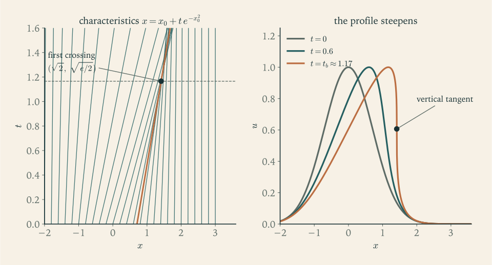
In Figure 2.1 the lines starting to the left of the crest spread apart, which flattens the back of the hump, while those starting just to the right of the crest converge. The crossing point is not at the crest: it is on the front face, on the characteristic that started where the initial profile was steepest.

2.4 After the break: shocks and the Rankine–Hugoniot condition

Past the breaking time the differential equation cannot hold everywhere, but the physical principle it came from still can. The integral conservation law of Section 1.2, in one dimension and without sources, says that for every interval \([a,b]\)

where \(\phi\) is the flux function, so that \(c=\phi'\) . This statement does not require \(u\) to be differentiable or even continuous. We therefore allow solutions with a jump across a curve, a shock, and ask what the conservation law demands of it.

The shock speed is thus the jump in flux divided by the jump in density. For the Burgers equation \(\phi(u)=u^2/2\) and

the average of the two states.

2.5 Which discontinuities are admissible

The two candidate solutions of the expansion problem differ in one respect. In the rarefaction every point is reached by a characteristic that can be traced back to the initial line. In the discontinuous candidate the characteristics on both sides emerge from the shock: on the left they have speed \(0<\tfrac12\) and on the right speed \(1>\tfrac12\) , so traced backward in time they run into the shock, not into the initial data. The values next to such a shock are not determined by the initial state. They are created at the discontinuity.

For a strictly convex flux, \(\phi''>0\) , the condition is equivalent to \(u_l>u_r\) : only downward jumps are allowed. The name comes from gas dynamics, where the condition expresses that entropy increases across a shock. For the Burgers equation the compression shock of Example 2.5 is admissible, since \(1>\tfrac12>0\) , and the expansion shock is not. It is a theorem, due to Oleinik for strictly convex fluxes and extended by Kruzhkov, and beyond the scope of this book, that for a strictly convex flux and bounded measurable initial data there is exactly one bounded weak solution that satisfies the entropy condition, the condition being stated for general bounded solutions as a one-sided bound on difference quotients. A piecewise smooth solution of the integral conservation law all of whose shocks are admissible in the sense of Definition 2.7 is that solution. We shall use the entropy condition as the selection rule and not prove that uniqueness theorem. Chapter 8 returns to shocks and shows how a discontinuous function can be said to satisfy a differential equation.

Exercises

1. Solve \(u_t+3u_x=0\) with \(u(x,0)=1/(1+x^2)\) , and find all points \(x\) at which \(u=\tfrac12\) when \(t=2\) .

   Answer

   \(u(x,t)=\dfrac{1}{1+(x-3t)^2}\) . At \(t=2\) the value \(\tfrac12\) is taken where \((x-6)^2=1\) , that is, at \(x=5\) and \(x=7\) .

2. Solve \(u_t+u_x=x\) with \(u(x,0)=0\) by integrating along characteristics, and verify the answer by substitution.

   Answer

   Along \(x=x_0+t\) we have \(z'=x_0+t\) , \(z(0)=0\) , so \(z=x_0t+\tfrac12t^2\) . With \(x_0=x-t\) this gives \(u(x,t)=xt-\tfrac12t^2\) . Check: \(u_t=x-t\) and \(u_x=t\) , so \(u_t+u_x=x\) .

3. Solve \(xu_x+yu_y=2u\) in the half-plane \(y>0\) with \(u(x,1)=g(x)\) , verify that the line \(y=1\) is noncharacteristic, and explain why the data on that line say nothing about the solution in the half-plane \(y<0\) .

   Solution

   The characteristic system is \(dx/ds=x\) , \(dy/ds=y\) , \(dz/ds=2z\) . Starting from the point \((r,1)\) of the data line with \(z=g(r)\) , the solutions are

   \[ x=re^{s},\qquad y=e^{s},\qquad z=g(r)e^{2s}. \]

   Eliminating the parameters, \(e^{s}=y\) and \(r=x/y\) , so \(u(x,y)=y^2g(x/y)\) for \(y>0\) . Check: \(u_x=y\,g'(x/y)\) and \(u_y=2y\,g(x/y)-x\,g'(x/y)\) , hence \(xu_x+yu_y=xyg'+2y^2g-xyg'=2u\) , and \(u(x,1)=g(x)\) .

   The data line is \((x_0,y_0)=(r,1)\) with tangent \((1,0)\) , and \(a\,y_0'-b\,x_0'=x\cdot 0-y\cdot 1=-1\ne 0\) on it, so it is noncharacteristic everywhere. The characteristics are the rays from the origin. A ray through a point of the line \(y=1\) has \(y=e^{s}>0\) for all \(s\) : it approaches the origin as \(s\to-\infty\) and never enters the lower half-plane. The rays in \(y<0\) meet no data, so there the solution is not determined; any function \(y^2h(x/y)\) solves the equation in \(y<0\) .

4. Find the characteristics of \(u_x+2xu_y=0\) , sketch them, and solve the equation with \(u(0,y)=\sin y\) .

   Answer

   The characteristics satisfy \(dy/dx=2x\) : they are the parabolas \(y=x^2+y_0\) , each crossing the \(y\) -axis once, at height \(y_0\) . Since \(u\) is constant on each, \(u(x,y)=\sin(y-x^2)\) .

5. Solve \(u_t+u_x=u^2\) with \(u(x,0)=g(x)\) by characteristics. For \(g(x)=1/(1+x^2)\) find the first time at which the solution becomes infinite and the point where this happens, and explain how this blow-up differs from the breaking described by Theorem 2.5.

   Solution

   The characteristics are the lines \(x=x_0+t\) , which are fixed in advance because the equation is semilinear. Along one of them \(z(t)=u(x_0+t,t)\) satisfies \(z'=z^2\) with \(z(0)=g(x_0)\) . Separating variables, \(-1/z=t-1/g(x_0)\) , so \(z=g(x_0)/(1-tg(x_0))\) and

   \[ u(x,t)=\frac{g(x-t)}{1-t\,g(x-t)} . \]

   The solution on the characteristic from \(x_0\) becomes infinite at the time \(t=1/g(x_0)\) if \(g(x_0)>0\) . The earliest such time is \(1/\max g\) . For \(g(x)=1/(1+x^2)\) the maximum is \(g(0)=1\) , so the first blow-up is at \(t=1\) on the characteristic from \(x_0=0\) , at the point \(x=1\) . Explicitly \(u=1/\bigl(1+(x-t)^2-t\bigr)\) , whose denominator first vanishes at \((x,t)=(1,1)\) .

   This is not the breaking of Theorem 2.5. There the characteristics cross, the solution stays bounded, and only its slope becomes infinite. Here the characteristics are parallel and never cross; the value of \(u\) itself runs off to infinity along a single characteristic because the ordinary differential equation \(z'=z^2\) blows up in finite time.

6. For the equation \(u_x+u_y=1\) consider data \(u(x,x)=g(x)\) on the line \(y=x\) . Show that the line is characteristic, that a solution exists only if \(g(x)=x+C\) for a constant \(C\) , and that in that case there are infinitely many solutions.

   Solution

   The equation has \((a,b)=(1,1)\) and the line \(y=x\) , parametrized by \((r,r)\) , has tangent \((1,1)\) ; so \(a\,y_0'-b\,x_0'=1-1=0\) and the line is characteristic. Along it, any \(C^1\) solution satisfies \(\tfrac{d}{dr}u(r,r)=u_x+u_y=1\) . Since \(u(r,r)=g(r)\) , a solution can exist only if \(g'(r)=1\) , that is, \(g(x)=x+C\) .

   To find all solutions put \(v=u-x\) ; then \(v_x+v_y=0\) , so \(v\) is constant on the lines \(y-x=\text{constant}\) and \(v=f(y-x)\) for a \(C^1\) function \(f\) . Hence \(u=x+f(y-x)\) , and on the line \(y=x\) this equals \(x+f(0)\) . If \(g(x)=x+C\) the data are matched by every \(f\) with \(f(0)=C\) : infinitely many solutions, for example \(u=x+C\) and \(u=x+C+(y-x)\) . If \(g\) is not of this form there is none. On a characteristic the equation already dictates how \(u\) varies, so the data are either inconsistent or redundant.

7. For the Burgers equation with \(u(x,0)=1/(1+x^2)\) find the breaking time \(t_b\) , the starting point \(x_0^{\ast}\) of the characteristic on which the solution breaks, and the location \(x_b\) of the break.

   Solution

   For the Burgers equation \(F=g\) with \(g(x)=(1+x^2)^{-1}\) , so \(g'(x)=-2x(1+x^2)^{-2}\) and

   \[ g''(x)=\frac{6x^2-2}{(1+x^2)^3}. \]

   The slope \(g'\) is most negative where \(g''=0\) with \(x>0\) , at \(x_0^{\ast}=1/\sqrt3\) . There \(1+x^2=\tfrac43\) and \(g'(x_0^{\ast})=-\dfrac{2}{\sqrt3}\cdot\dfrac{9}{16}=-\dfrac{3\sqrt3}{8}\) . By Theorem 2.5 the breaking time is

   \[ t_b=\frac{8}{3\sqrt3}=\frac{8\sqrt3}{9}\approx 1.540 . \]

   The characteristic from \(x_0^{\ast}\) carries the value \(g(x_0^{\ast})=\tfrac34\) , so the break occurs at \(x_b=x_0^{\ast}+t_b\cdot\tfrac34=\dfrac{1}{\sqrt3}+\dfrac{2}{\sqrt3}=\sqrt3\) . The hypotheses of the theorem hold because \(g\) and \(g'\) are bounded and the infimum of \(g'\) is attained.

8. Show that the Burgers equation with \(u(x,0)=\arctan x\) has a classical solution for all \(t\ge 0\) whose slope \(u_x\) tends to zero as \(t\to\infty\) at every point, while with \(u(x,0)=-\arctan x\) the solution breaks at \(t=1\) at the point \(x=0\) .

   Hint

   Use \(u_x=g'(x_0)/(1+tg'(x_0))\) . For \(g=\arctan\) , \(g'(x_0)=1/(1+x_0^2)>0\) , so \(m\ge 0\) and \(u_x=1/(1+x_0^2+t)\le 1/t\) . For \(g=-\arctan\) the slope \(g'\) is most negative at \(x_0=0\) , where it equals \(-1\) , so \(t_b=1\) ; the characteristic from \(x_0=0\) carries the value \(0\) and stays at \(x=0\) .

9. For the traffic model of Example 2.6 with general \(v_m\) and \(\rho_m\) , let the initial density be \(\rho(x,0)=\tfrac12\rho_m\bigl(1+\tanh(x/\ell)\bigr)\) , light traffic running into heavy traffic over a transition length \(\ell\) . Compute \(F=\phi'\circ\rho(\cdot,0)\) , find the breaking time, and evaluate it for \(v_m=25\ \mathrm{m/s}\) and \(\ell=100\ \mathrm{m}\) .

   Answer

   \(F(x)=v_m\bigl(1-2\rho(x,0)/\rho_m\bigr)=-v_m\tanh(x/\ell)\) , so \(F'(x)=-(v_m/\ell)\operatorname{sech}^2(x/\ell)\) with minimum \(m=-v_m/\ell\) at \(x=0\) . The breaking time is \(t_b=\ell/v_m\) , which is \(4\ \mathrm{s}\) for the given values. A gradual transition into heavy traffic sharpens into a jump.

10. For the Burgers equation with \(u=3\) for \(x<0\) and \(u=1\) for \(x>0\) , find the shock speed and position, check the entropy condition, and verify the integral conservation law directly on the interval \([-10,10]\) at a time \(t<5\) .

    Answer

    \(\sigma'=(3+1)/2=2\) , so the shock is at \(x=2t\) ; it is admissible since \(3>2>1\) . For \(t<5\) , \(\int_{-10}^{10}u\,dx=3(2t+10)+(10-2t)=40+4t\) , with rate of change \(4\) , and \(\phi(3)-\phi(1)=\tfrac92-\tfrac12=4\) .

11. A student argues: “In \(u_t+xu_x=0\) the speed at the point \(x\) is \(x\) , so by Theorem 2.1 the solution with \(u(x,0)=g(x)\) is \(u=g(x-xt)\) .” Substitute this formula into the equation to show it is wrong, identify the step of the argument that fails, and give the correct solution.

    Solution

    Let \(u=g(x-xt)=g\bigl(x(1-t)\bigr)\) . Then \(u_t=-x\,g'\) and \(u_x=(1-t)\,g'\) , with \(g'\) evaluated at \(x(1-t)\) , so

    \[ u_t+xu_x=-xg'+x(1-t)g'=-xt\,g' , \]

    which is not zero unless \(g\) is constant. The formula is wrong.

    The failing step is the appeal to Theorem 2.1, which assumes a constant speed. The student treated a particle arriving at \(x\) at time \(t\) as if it had travelled at the speed \(x\) all along and so had started at \(x-xt\) . But the speed is the particle’s current position, which changes as it moves: the path satisfies \(dx/dt=x\) , so \(x=x_0e^{t}\) , an exponential and not a straight line. Inverting, \(x_0=xe^{-t}\) , and since \(u\) is constant on each path the correct solution is \(u=g(xe^{-t})\) , as in Example 2.2. The two formulas agree to first order in \(t\) , because \(e^{-t}=1-t+\dots\) , which is why the wrong one looks plausible for small times.

12. Solve the Riemann problem for the Burgers equation with \(u_l=1\) and \(u_r=3\) by a rarefaction wave, and show that the alternative solution consisting of a single shock satisfies the Rankine–Hugoniot condition and violates the entropy condition.

    Answer

    Rarefaction: \(u=1\) for \(x\le t\) , \(u=x/t\) for \(t<x<3t\) , \(u=3\) for \(x\ge 3t\) ; it is continuous for \(t>0\) and solves the equation in each region. The single shock \(u=1\) for \(x<2t\) , \(u=3\) for \(x>2t\) has the Rankine–Hugoniot speed \((1+3)/2=2\) , but \(\phi'(u_l)=1<2<3=\phi'(u_r)\) , the reverse of the entropy inequalities: characteristics leave the shock on both sides.

13. For the Burgers equation with \(u(x,0)=1\) for \(0<x<1\) and \(u(x,0)=0\) elsewhere, find the entropy solution for all \(t>0\) : describe the rarefaction and the shock for \(t<2\) , show that the rarefaction overtakes the shock at \(t=2\) , and find the shock path and the height of the solution for \(t>2\) . Check that \(\int u\,dx\) is conserved.

    Solution

    Early times. At \(x=0\) the data jump upward from \(0\) to \(1\) , which is not an admissible shock, so a rarefaction opens: \(u=x/t\) for \(0<x<t\) . At \(x=1\) the data jump downward from \(1\) to \(0\) , an admissible shock with speed \((1+0)/2=\tfrac12\) , located at \(\sigma(t)=1+\tfrac12t\) . So for \(t<2\)

    \[ u=0\ (x<0),\qquad u=\frac xt\ (0<x<t),\qquad u=1\ (t<x<1+\tfrac12t),\qquad u=0\ (x>1+\tfrac12t). \]

    The leading edge of the rarefaction, \(x=t\) , moves at speed \(1\) and the shock at speed \(\tfrac12\) ; they meet when \(t=1+\tfrac12t\) , that is, at \(t=2\) and \(x=2\) .

    Late times. For \(t>2\) the state just left of the shock is the rarefaction value \(u_l=\sigma/t\) , and \(u_r=0\) . The Rankine–Hugoniot condition gives \(\sigma'=\sigma/(2t)\) , whose solutions are \(\sigma=C\sqrt t\) ; matching \(\sigma(2)=2\) gives \(C=\sqrt2\) , so

    \[ \sigma(t)=\sqrt{2t},\qquad u=\frac xt\ \text{ for }0<x<\sqrt{2t},\qquad u=0\ \text{ otherwise}. \]

    The height at the shock is \(\sigma/t=\sqrt{2/t}\) , which decays, and the shock is admissible since \(u_l>0=u_r\) .

    Conservation. For \(t<2\) the integral is \(\tfrac12t\cdot 1+\bigl(1+\tfrac12t-t\bigr)\cdot 1=1\) . For \(t>2\) the profile is a triangle of base \(\sqrt{2t}\) and height \(\sqrt{2/t}\) with area \(\tfrac12\sqrt{2t}\sqrt{2/t}=1\) . The total is conserved, as the integral law demands with zero flux at both ends.

14. In the green-light solution of Example 2.6, a car waits at \(x=-L\) . Use the velocity law \(v=v_m(1-\rho/\rho_m)\) and the rarefaction formula to write the differential equation for the car’s position once the fan reaches it, solve it, and find when the car passes the light. Evaluate for \(L=100\ \mathrm{m}\) and \(v_m=25\ \mathrm{m/s}\) .

    Solution

    The rear edge of the fan, \(x=-v_mt\) , reaches the car at \(t_0=L/v_m\) . From then on the car is inside the fan, where \(\rho/\rho_m=\tfrac12\bigl(1-x/(v_mt)\bigr)\) , so its velocity is

    \[ \frac{dx}{dt}=v_m\left(1-\frac{\rho}{\rho_m}\right)=\frac{v_m}{2}+\frac{x}{2t},\qquad x(t_0)=-L . \]

    This is a linear first-order equation. Put \(x=v_mt+w\) ; then \(w'=w/(2t)\) , so \(w=C\sqrt t\) . The initial condition \(-L=L+C\sqrt{L/v_m}\) gives \(C=-2\sqrt{Lv_m}\) , hence

    \[ x(t)=v_mt-2\sqrt{Lv_mt}\qquad(t\ge L/v_m). \]

    Check: \(x'=v_m-\sqrt{Lv_m/t}\) , and \(\tfrac12v_m+x/(2t)=v_m-\sqrt{Lv_m/t}\) as well. The car passes the light when \(x=0\) , that is, when \(v_mt=2\sqrt{Lv_mt}\) , so \(t=4L/v_m\) . For \(L=100\ \mathrm{m}\) and \(v_m=25\ \mathrm{m/s}\) the car starts to move at \(t_0=4\ \mathrm{s}\) and passes the light at \(t=16\ \mathrm{s}\) , four times as long as the wait before it could move at all.

15. Classify each first-order equation as linear, semilinear, or quasilinear in the sense of Definition 1.2 and say whether its characteristics can be drawn before the solution is known: (a) \(u_t+xu_x=0\) ; (b) \(u_t+u_x=u^2\) ; (c) \(u_t+uu_x=0\) ; (d) \(u_t+(1-2u)u_x=0\) .

    Answer

    (a) Linear; the characteristics \(x=x_0e^{t}\) are known in advance. (b) Semilinear; the characteristics \(x=x_0+t\) are known in advance, and only the values along them depend on the solution. (c) and (d) Quasilinear; the coefficient of \(u_x\) depends on \(u\) , so the characteristics depend on the data and cannot be drawn until the solution is known along them.

16. Let \(u\) be a \(C^2\) solution of the Burgers equation and let \(w=u_x\) . Differentiate the equation in \(x\) to show that along each characteristic \(dw/dt=-w^2\) , solve this equation, and recover the formula for \(u_x\) in Theorem 2.5 together with the breaking time.

    Solution

    Differentiating \(u_t+uu_x=0\) with respect to \(x\) gives \(u_{xt}+u_x^2+uu_{xx}=0\) , that is, \(w_t+uw_x=-w^2\) . A characteristic is a curve with \(dx/dt=u\) , and along it \(\tfrac{d}{dt}w(x(t),t)=w_t+uw_x\) . Therefore

    \[ \frac{dw}{dt}=-w^2\qquad\text{along each characteristic.} \]

    This Riccati equation separates: \(\tfrac{d}{dt}(1/w)=1\) , so \(1/w=t+1/w_0\) and \(w=w_0/(1+tw_0)\) , where \(w_0=g'(x_0)\) is the initial slope at the foot of the characteristic. This is the formula \(u_x=g'(x_0)/(1+tF'(x_0))\) of Theorem 2.5 with \(F=g\) . If \(w_0\ge 0\) the slope decays like \(1/t\) . If \(w_0<0\) the slope becomes infinite at \(t=-1/w_0\) , and the earliest such time over all characteristics is \(-1/\min g'\) , the breaking time. The argument assumed \(u\in C^2\) so that \(w\) could be differentiated; the theorem needs only \(C^1\) data.

17. Verify that \(u(x,t)=\int_0^tf\bigl(x-c(t-s),s\bigr)ds\) solves \(u_t+cu_x=f\) with \(u(x,0)=0\) when \(f\) and \(f_x\) are continuous, and evaluate the formula for \(c=1\) and \(f(x,t)=\cos x\) .

    Hint

    Differentiate under the integral sign: \(u_t=f(x,t)+\int_0^t(-c)f_x\bigl(x-c(t-s),s\bigr)ds\) and \(u_x=\int_0^tf_x\bigl(x-c(t-s),s\bigr)ds\) . For the example, \(u=\int_0^t\cos(x-t+s)\,ds=\sin x-\sin(x-t)\) .