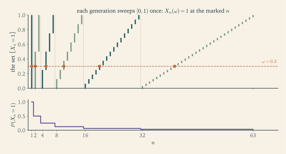
Cut \([0,1)\) into halves, then quarters, then eighths, and list the pieces in order: \([0,1)\) ; \([0,\tfrac12)\) , \([\tfrac12,1)\) ; \([0,\tfrac14)\) , \([\tfrac14,\tfrac12)\) , and so on. Let \(X_n\) be the indicator of the \(n\) -th piece in the list, regarded as a random variable on \([0,1)\) with Lebesgue measure. As \(n\) grows the pieces shrink, so the probability that \(X_n\) is not zero tends to \(0\) ; for large \(n\) one would bet heavily that \(X_n=0\) . And yet at every single sample point \(\omega\) the sequence \(X_n(\omega)\) takes the value \(1\) infinitely often, once in each round of subdivision, and the value \(0\) infinitely often. As a sequence of numbers it converges for no \(\omega\) at all.
Does this sequence converge to zero? The question has no answer until “converge” is given a meaning, and probability uses four. They differ in what they look at: the path \(n\mapsto X_n(\omega)\) for each fixed \(\omega\) , the probability of a noticeable error at each fixed \(n\) , the average size of the error, or only the law of \(X_n\) . This chapter defines the four modes, proves every implication that holds among them, gives a counterexample for every implication that fails, and then proves the partial converses that make the weaker modes usable. The sequence above, which we shall call the typewriter sequence because its carriage sweeps across the interval and returns, is the most important of the counterexamples.
4.1 Four definitions
Definition 4.1 (modes of convergence). Let \(X,X_1,X_2,\dots\) be random variables on one probability space.
The sequence converges to \(X\) almost surely, written \(X_n\to X\) a.s., if \(\mathbb P(\{\omega:X_n(\omega)\to X(\omega)\})=1\) .
It converges in probability, written \(X_n\xrightarrow{\ \mathbb P\ }X\) , if \(\mathbb P(\lvert X_n-X\rvert>\varepsilon)\to 0\) for every \(\varepsilon>0\) .
It converges in \(L^p\) , for a given \(p>0\) , written \(X_n\xrightarrow{L^p}X\) , if all the variables belong to \(L^p\) and \(\mathbb E\lvert X_n-X\rvert^p\to 0\) .
It converges in distribution, written \(X_n\xrightarrow{\ d\ }X\) , if \(\mathbb E f(X_n)\to\mathbb E f(X)\) for every bounded continuous \(f:\mathbb R\to\mathbb R\) .
The fourth definition involves each \(X_n\) only through \(\mathbb E f(X_n)\) , which by Theorem 1.11 is a functional of the law of \(X_n\) . Convergence in distribution is therefore a statement about a sequence of laws; the variables need not even be defined on the same sample space. Chapter 9 studies it in its own right and shows that it is equivalent to convergence of the distribution functions at every point where the limit is continuous. In this chapter it appears only as the weakest of the four.
The first two definitions differ in the placement of a quantifier. Almost sure convergence fixes \(\omega\) first and asks the whole sequence \(X_n(\omega)\) to settle. Convergence in probability fixes \(n\) first and asks the set of \(\omega\) at which \(X_n\) is far from \(X\) to be small; that set may be a different one for every \(n\) , and it may wander over the whole sample space, as the pieces of the typewriter sequence do. The following lemma puts the two on the same footing.
Lemma 4.2 (almost sure convergence through tail suprema). For random variables \(X,X_1,X_2,\dots\) the following are equivalent: (a) \(X_n\to X\) almost surely; (b) \(\mathbb P(\lvert X_n-X\rvert>\varepsilon\ \text{i.o.})=0\) for every \(\varepsilon>0\) ; (c) \(\mathbb P(\sup_{k\ge n}\lvert X_k-X\rvert>\varepsilon)\to 0\) as \(n\to\infty\) , for every \(\varepsilon>0\) .
Proof. A sequence of numbers fails to converge to \(x\) exactly when, for some \(j\ge 1\) , it is at distance more than \(1/j\) from \(x\) infinitely often. So
and a countable union of events is null exactly when each of them is. Since the events in (b) increase as \(\varepsilon\) decreases, this gives the equivalence of (a) and (b). For (c), fix \(\varepsilon\) and let \(B_n=\{\sup_{k\ge n}\lvert X_k-X\rvert>\varepsilon\}=\bigcup_{k\ge n}\{\lvert X_k-X\rvert>\varepsilon\}\) . The events \(B_n\) decrease to \(\{\lvert X_k-X\rvert>\varepsilon\ \text{i.o.}\}\) , so their probabilities tend to the probability of that event, which is \(0\) if and only if (b) holds for this \(\varepsilon\) .
Condition (c) is the comparison to remember: almost sure convergence asks that the largest error from time \(n\) onward be small with high probability, while convergence in probability asks this only of the error at time \(n\) . Condition (b), combined with the first Borel–Cantelli lemma, gives the standard sufficient condition: if \(\sum_n\mathbb P(\lvert X_n-X\rvert>\varepsilon)<\infty\) for every \(\varepsilon>0\) , then \(X_n\to X\) almost surely.
4.2 The implications that hold
Theorem 4.3 (implications among the modes). Let \(X,X_1,X_2,\dots\) be random variables on one probability space.
(i) If \(X_n\to X\) almost surely, then \(X_n\to X\) in probability.
(ii) If \(X_n\to X\) in \(L^p\) for some \(p>0\) , then \(X_n\to X\) in probability.
(iii) If \(X_n\to X\) in \(L^q\) and \(0<p\le q\) , then \(X_n\to X\) in \(L^p\) .
(iv) If \(X_n\to X\) in probability, then \(X_n\to X\) in distribution.
Proof. (i) For each \(\varepsilon>0\) , \(\mathbb P(\lvert X_n-X\rvert>\varepsilon)\le\mathbb P(\sup_{k\ge n}\lvert X_k-X\rvert>\varepsilon)\) , and the right side tends to \(0\) by Lemma 4.2.
(ii) By Markov’s inequality, \(\mathbb P(\lvert X_n-X\rvert>\varepsilon)\le\varepsilon^{-p}\,\mathbb E\lvert X_n-X\rvert^p\to 0\) .
(iii) By Lyapunov’s inequality (Corollary 1.15), \(\lVert X_n-X\rVert_p\le\lVert X_n-X\rVert_q\to 0\) .
(iv) Let \(f\)
be bounded and continuous with \(\lvert f\rvert\le M\)
, and let \(\varepsilon>0\)
. Choose \(K\)
so large that \(\mathbb P(\lvert X\rvert>K)\le\varepsilon\)
. On the compact interval \([-K-1,K+1]\)
the function \(f\)
is uniformly continuous, by the Heine–Cantor theorem of Real Analysis (math.real-analysis.heine-cantor), so there is \(\delta\in(0,1)\)
with \(\lvert f(x)-f(y)\rvert\le\varepsilon\)
whenever \(\lvert x\rvert\le K\)
and \(\lvert x-y\rvert\le\delta\)
. On the event \(\{\lvert X\rvert\le K\}\cap\{\lvert X_n-X\rvert\le\delta\}\)
we therefore have \(\lvert f(X_n)-f(X)\rvert\le\varepsilon\)
, and on its complement \(\lvert f(X_n)-f(X)\rvert\le 2M\)
. Hence
Letting \(n\to\infty\) and then \(\varepsilon\to 0\) gives \(\mathbb E f(X_n)\to\mathbb E f(X)\) .
These four arrows are the solid arrows of Figure 4.1, and no others hold in general. Convergence in probability sits in the middle: it follows from each of the two strong modes and implies the weak one. The two strong modes, almost sure and \(L^p\) , are not comparable.

4.3 The implications that fail
Each missing arrow of Figure 4.1 is ruled out by an example, and each example isolates one mechanism. They are worth knowing by name.
Example 4.1: The typewriter sequence
Every integer \(n\ge 1\) can be written uniquely as \(n=2^k+j\) with \(k\ge 0\) and \(0\le j<2^k\) . On \(([0,1),\mathcal B,\lambda)\) let
Thus \(X_1\) is the indicator of \([0,1)\) , \(X_2\) and \(X_3\) of the two halves, \(X_4,\dots,X_7\) of the four quarters. The indices \(2^k\le n<2^{k+1}\) form the \(k\) -th generation.
Convergence in probability and in every \(L^p\) . For \(n\) in generation \(k\) and \(0<\varepsilon<1\) , \(\mathbb P(\lvert X_n\rvert>\varepsilon)=2^{-k}\) , and \(\mathbb E\lvert X_n\rvert^p=2^{-k}\) for every \(p>0\) , because \(X_n^p=X_n\) . As \(n\to\infty\) the generation \(k\) tends to infinity, so \(X_n\to 0\) in probability and in \(L^p\) for every \(p\) .
No almost sure convergence. Fix \(\omega\in[0,1)\) . The intervals of generation \(k\) partition \([0,1)\) , so exactly one of them contains \(\omega\) : in each generation \(X_n(\omega)=1\) for one index and \(X_n(\omega)=0\) for the other \(2^k-1\) . For \(\omega=0.3\) the indices with \(X_n(\omega)=1\) are \(n=1,2,5,10,20,41,\dots\) , one in each generation. Hence \(\limsup_nX_n(\omega)=1\) and \(\liminf_nX_n(\omega)=0\) for every \(\omega\) , and the set of convergence is empty. In the terms of Lemma 4.2, \(\sup_{m\ge n}X_m=1\) everywhere, so \(\mathbb P(\sup_{m\ge n}\lvert X_m\rvert>\tfrac12)=1\) for all \(n\) although \(\mathbb P(\lvert X_n\rvert>\tfrac12)\to 0\) .
The mechanism is a small exceptional set that moves. Convergence in probability and in \(L^p\) see only its size; almost sure convergence sees that it visits every point again and again.
Example 4.2: The escaping spike
On \(((0,1),\mathcal B,\lambda)\) let \(X_n=n\,\mathbf 1_{(0,1/n)}\) . For each fixed \(\omega\) , \(X_n(\omega)=0\) as soon as \(n\ge 1/\omega\) , so \(X_n\to 0\) at every sample point, hence almost surely and in probability. But
so \(X_n\) does not converge to \(0\) in \(L^1\) , and it cannot converge in \(L^1\) to anything else, since an \(L^1\) limit would also be a limit in probability. Almost sure convergence does not imply convergence in \(L^1\) , and the expectations \(\mathbb E X_n=1\) do not converge to the expectation \(0\) of the limit.
Varying the height separates the \(L^p\) spaces from each other. For \(Y_n=n^{a}\mathbf 1_{(0,1/n)}\) with \(a>0\) , \(\mathbb E\,Y_n^p=n^{ap-1}\) , which tends to \(0\) exactly when \(ap<1\) . With \(a=1/2\) : \(\mathbb E\,Y_n=n^{-1/2}\to 0\) while \(\mathbb E\,Y_n^2=1\) , so \(Y_n\to 0\) in \(L^1\) and not in \(L^2\) .
The mechanism is a small set carrying a large value: probability \(1/n\) times height \(n\) is a fixed amount of expectation that escapes to infinity. Chapter 5 is devoted to excluding exactly this.
Example 4.3: Same laws, opposite variables
Let \(X\) take the values \(1\) and \(-1\) with probability \(1/2\) each, and let \(X_n=(-1)^nX\) . Every \(X_n\) has the same law as \(X\) , so \(\mathbb E f(X_n)=\mathbb E f(X)\) for every \(f\) and all \(n\) , and \(X_n\to X\) in distribution trivially. But for odd \(n\) , \(\lvert X_n-X\rvert=2\lvert X\rvert=2\) at every sample point, so \(\mathbb P(\lvert X_n-X\rvert>1)=1\) for odd \(n\) and \(X_n\) does not converge to \(X\) in probability. It does not converge in probability to any random variable: if it did, the differences \(X_{n+1}-X_n\) would tend to \(0\) in probability, whereas \(\lvert X_{n+1}-X_n\rvert=2\) always.
The mechanism is that convergence in distribution knows nothing of the coupling between \(X_n\) and \(X\) . The same conclusion holds for any i.i.d. sequence with a nondegenerate law: it converges in distribution, having constant law, and not in probability.
Example 4.4: Two sequences with the same marginal laws
Let \(U\) be uniform on \((0,1)\) and set \(X_n'=\mathbf 1_{\{U<1/n\}}\) . Separately, let \(A_1,A_2,\dots\) be independent events with \(\mathbb P(A_n)=1/n\) and set \(X_n=\mathbf 1_{A_n}\) . For each \(n\) the variables \(X_n\) and \(X_n'\) have the same law: both equal \(1\) with probability \(1/n\) and \(0\) otherwise. Both sequences converge to \(0\) in probability and in every \(L^p\) , since these statements involve only the law of each term.
Almost sure convergence distinguishes them. The sets \(\{U<1/n\}\) decrease, so \(X_n'(\omega)=0\) for all \(n\ge 1/U(\omega)\) and \(X_n'\to 0\) at every sample point. For the independent sequence, \(\sum_n\mathbb P(A_n)=\infty\) and the second Borel–Cantelli lemma gives \(X_n=1\) infinitely often almost surely, so \(X_n\) converges with probability \(0\) (Exercise 3.18). The tail suprema of Lemma 4.2 make the difference quantitative. For \(2\le n\le N\) ,
Letting \(N\to\infty\) : \(\mathbb P(\sup_{k\ge n}X_k'>\tfrac12)=\tfrac1n\to 0\) , while \(\mathbb P(\sup_{k\ge n}X_k>\tfrac12)=1\) for every \(n\) .
So almost sure convergence is a property of the joint law of the entire sequence, and cannot be read from the laws of its terms. This is the precise sense in which the sample space of Section 1.5 matters.
4.4 Partial converses
The weaker modes would be of little use if nothing could be recovered from them. Three results recover a good deal: convergence in probability gives almost sure convergence along a subsequence; that fact characterizes convergence in probability and transfers to it most of the calculus of almost sure limits; and convergence in distribution to a constant is convergence in probability.
Theorem 4.4 (almost sure convergence along a subsequence). If \(X_n\to X\) in probability, there is a subsequence \(n_1<n_2<\cdots\) with \(X_{n_k}\to X\) almost surely.
Proof. Since \(\mathbb P(\lvert X_n-X\rvert>2^{-k})\to 0\) as \(n\to\infty\) for each \(k\) , we can choose \(n_1<n_2<\cdots\) with \(\mathbb P(\lvert X_{n_k}-X\rvert>2^{-k})\le 2^{-k}\) . These probabilities are summable, so by the first Borel–Cantelli lemma, almost surely \(\lvert X_{n_k}-X\rvert\le 2^{-k}\) for all but finitely many \(k\) , and on that event \(X_{n_k}\to X\) .
For the typewriter sequence the subsequence \(n_k=2^k\) works: \(X_{2^k}\) is the indicator of \([0,2^{-k})\) , which tends to \(0\) at every \(\omega>0\) .
Theorem 4.5 (subsequence criterion). \(X_n\to X\) in probability if and only if every subsequence of \((X_n)\) has a further subsequence that converges to \(X\) almost surely.
Proof. If \(X_n\to X\) in probability, so does every subsequence, and Theorem 4.4 applied to the subsequence gives the further subsequence. Conversely, suppose \(X_n\) does not converge to \(X\) in probability. Then there are \(\varepsilon>0\) , \(\delta>0\) , and a subsequence \((n_k)\) with \(\mathbb P(\lvert X_{n_k}-X\rvert>\varepsilon)\ge\delta\) for all \(k\) . No further subsequence of it can converge to \(X\) almost surely, because by Theorem 4.3(i) it would then converge in probability, which the lower bound \(\delta\) forbids.
The criterion reduces questions about convergence in probability to questions about almost sure convergence, where one can argue pointwise. It combines well with an elementary fact about numbers: a real sequence \(a_n\)
converges to \(a\)
if and only if every subsequence has a further subsequence converging to \(a\)
. The corollary below uses the Dominated Convergence Theorem of Measure Theory in its standard form: if \(Z_n\to Z\)
almost surely and \(\lvert Z_n\rvert\le Y\)
for an integrable \(Y\)
, then \(\mathbb E\lvert Z_n-Z\rvert\to 0\)
(math.measure-theory.dominated-convergence-theorem).
Corollary 4.6 (calculus of limits in probability). Suppose \(X_n\to X\) and \(Y_n\to Y\) in probability.
(a) The limit is unique: if also \(X_n\to X'\) in probability, then \(X=X'\) almost surely.
(b) If \(g:\mathbb R^2\to\mathbb R\) is continuous, then \(g(X_n,Y_n)\to g(X,Y)\) in probability. In particular \(X_n+Y_n\to X+Y\) and \(X_nY_n\to XY\) in probability.
(c) If \(\lvert X_n\rvert\le Z\) for all \(n\) , where \(Z\) is integrable, then \(X\) is integrable and \(\mathbb E\lvert X_n-X\rvert\to 0\) ; in particular \(\mathbb E X_n\to\mathbb E X\) .
Proof. (a) A subsequence converges almost surely to \(X\) , and a further subsequence converges almost surely to \(X'\) ; limits of numerical sequences are unique.
(b) Given any subsequence, extract a further subsequence along which \(X_n\to X\) almost surely, and from that another along which also \(Y_n\to Y\) almost surely. Along it \(g(X_n,Y_n)\to g(X,Y)\) almost surely by continuity. Theorem 4.5 gives the claim.
(c) Along an almost surely convergent subsequence \(\lvert X\rvert=\lim\lvert X_{n_k}\rvert\le Z\) , so \(X\) is integrable. Let \(a_n=\mathbb E\lvert X_n-X\rvert\) . Every subsequence of \((a_n)\) has a further subsequence along which \(X_n\to X\) almost surely, and along that one \(a_n\to 0\) by the Dominated Convergence Theorem with dominating function \(2Z\) . Hence \(a_n\to 0\) .
Part (c) says that the Dominated Convergence Theorem holds with convergence in probability in place of almost sure convergence. The typewriter sequence shows that the subsequence criterion has no analogue for almost sure convergence itself: every subsequence of it has a further subsequence converging to \(0\) almost surely, by Theorem 4.5, and yet the sequence converges nowhere. In a metric space, or in any topological space, a sequence all of whose subsequences have further subsequences converging to a point converges to that point. So there is no metric and no topology on random variables for which convergence means almost sure convergence. Convergence in probability, by contrast, comes from a metric.
Theorem 4.7 (convergence in distribution to a constant). If \(X_n\to c\) in distribution, where \(c\) is a constant, then \(X_n\to c\) in probability.
Proof. Fix \(\varepsilon>0\) and let \(f(x)=\min(\lvert x-c\rvert/\varepsilon,1)\) , a bounded continuous function with \(f(c)=0\) and \(f(x)=1\) when \(\lvert x-c\rvert\ge\varepsilon\) . Then \(\mathbb P(\lvert X_n-c\rvert\ge\varepsilon)\le\mathbb E f(X_n)\to f(c)=0\) .
The constant limit is what makes this work: a constant has only one coupling with any other variable, so the information that convergence in distribution lacks is not needed.
Theorem 4.8 (a complete metric for convergence in probability). For random variables \(X\) and \(Y\) on one probability space let
Then \(d\) is a metric on random variables identified when almost surely equal; \(X_n\to X\) in probability if and only if \(d(X_n,X)\to 0\) ; and the metric is complete: if \(d(X_m,X_n)\to 0\) as \(m,n\to\infty\) , there is a random variable \(X\) with \(X_n\to X\) in probability.
Proof. Symmetry is clear, \(d(X,Y)=0\) exactly when \(X=Y\) almost surely, and the triangle inequality follows from \(\lvert x-z\rvert\wedge 1\le\lvert x-y\rvert\wedge 1+\lvert y-z\rvert\wedge 1\) . For \(0<\varepsilon\le 1\) and any random variable \(Z\) ,
the first inequality by Markov and the second by splitting the expectation according to whether \(\lvert Z\rvert\le\varepsilon\) . With \(Z=X_n-X\) these give the second claim.
For completeness, let \((X_n)\) be a Cauchy sequence for \(d\) . Choose \(n_1<n_2<\cdots\) so that \(d(X_m,X_{n_k})\le 4^{-k}\) for all \(m\ge n_k\) . By the left inequality with \(\varepsilon=2^{-k}\) , \(\mathbb P(\lvert X_{n_{k+1}}-X_{n_k}\rvert>2^{-k})\le 2^{-k}\) . By the first Borel–Cantelli lemma, almost surely \(\lvert X_{n_{k+1}}-X_{n_k}\rvert\le 2^{-k}\) for all large \(k\) , so the series \(\sum_k(X_{n_{k+1}}-X_{n_k})\) converges absolutely and \(X_{n_k}\) converges almost surely. Let \(X\) be the limit where it exists and \(0\) elsewhere. Then \(X_{n_k}\to X\) almost surely, hence in probability, so \(d(X_{n_k},X)\to 0\) by the second claim; and \(d(X_n,X)\le d(X_n,X_{n_k})+d(X_{n_k},X)\le 4^{-k}+d(X_{n_k},X)\) for \(n\ge n_k\) shows that the whole sequence converges.
The spaces \(L^p\)
with \(p\ge 1\)
are complete as well; that is the Riesz–Fischer theorem of Measure Theory (math.measure-theory.lp-completeness), and its proof uses the same device of a rapidly converging subsequence.
Example 4.5: The metric evaluated on the counterexamples
For the spike \(X_n=n\mathbf 1_{(0,1/n)}\) of Example 4.2 and \(n\ge 1\) , \(\lvert X_n\rvert\wedge 1=\mathbf 1_{(0,1/n)}\) , so
Truncating at \(1\) is exactly what stops the metric from seeing the height of the spike. For the typewriter sequence in generation \(k\) , \(d(X_n,0)=2^{-k}\to 0\) . For the sequence \(X_n=(-1)^nX\) of Example 4.3, \(\lvert X_n-X\rvert\) equals \(2\) for odd \(n\) and \(0\) for even \(n\) , so \(d(X_n,X)\) alternates between \(1\) and \(0\) and does not converge.
The two-sided bound in the proof of Theorem 4.8 can be checked on the spike with \(\varepsilon=\tfrac12\) : \(\mathbb P(\lvert X_n\rvert>\tfrac12)=\tfrac1n\) , and indeed \(\tfrac12\cdot\tfrac1n\le\tfrac1n\le\tfrac12+\tfrac1n\) .
Common mistake. Reversing an arrow of Figure 4.1. Two reversals account for most errors. The first: “\(\mathbb P(\lvert X_n-X\rvert>\varepsilon)\to 0\) , so for almost every \(\omega\) the numbers \(X_n(\omega)\) approach \(X(\omega)\) .” The typewriter sequence refutes it; what is true is the statement for a subsequence, or for the full sequence when the probabilities are summable. The second: “\(X_n\to X\) almost surely, so \(\mathbb E X_n\to\mathbb E X\) .” The spike refutes it; what is true needs domination, as in Corollary 4.6(c), or the uniform integrability of Chapter 5. A practical habit is to write the mode over every arrow and to attach to each inference the theorem that licenses it.
4.5 What each mode supports
The modes are not ranked by strength alone; each permits different operations.
| Mode | What it depends on | Continuous functions | Expectations |
|---|---|---|---|
| almost surely | the joint law of the whole sequence and the limit | preserved, pointwise | converge only with extra control, such as domination |
| in probability | the joint law of each pair \((X_n,X)\) | preserved, by Corollary 4.6 | converge only with extra control; Chapter 5 gives the exact condition |
| in \(L^p\) | the joint law of each pair \((X_n,X)\) | preserved for Lipschitz functions | \(\mathbb E\lvert X_n\rvert^p\to\mathbb E\lvert X\rvert^p\) , and \(\mathbb E X_n\to\mathbb E X\) when \(p\ge 1\) |
| in distribution | the law of each \(X_n\) and of \(X\) | preserved; proved in Chapter 9 | converge for bounded continuous functions of \(X_n\) |
Reading down the second column explains the counterexamples. A mode can only be implied by modes that depend on at least as much information, and it can be broken by changing information it depends on while leaving the rest alone: Example 4.4 changed the joint law of the sequence without changing any marginal law, and Example 4.3 changed the coupling with the limit without changing any law at all.
Laws of large numbers come in a weak form and a strong form, and the difference between them is the difference between the second row and the first. Before those theorems, two tools are still missing. The spike showed that expectations can fail to converge even under almost sure convergence. What is the exact condition under which they do converge?
Exercises
-
Prove that limits in probability are almost surely unique directly from the definition, by bounding \(\mathbb P(\lvert X-X'\rvert>2\varepsilon)\) , without using subsequences.
Hint
If \(\lvert X-X'\rvert>2\varepsilon\) then \(\lvert X_n-X\rvert>\varepsilon\) or \(\lvert X_n-X'\rvert>\varepsilon\) , so \(\mathbb P(\lvert X-X'\rvert>2\varepsilon)\le\mathbb P(\lvert X_n-X\rvert>\varepsilon)+\mathbb P(\lvert X_n-X'\rvert>\varepsilon)\) for every \(n\) . The left side does not depend on \(n\) .
-
Suppose \(X_n\to X\) in \(L^2\) . Prove that \(\mathbb E X_n\to\mathbb E X\) and \(\mathbb E X_n^2\to\mathbb E X^2\) , and compute both differences explicitly for \(X=U\) and \(X_n=U+U^{-1/4}/n\) with \(U\) uniform on \((0,1)\) .
Solution
For the means, Lyapunov’s inequality gives \(\lvert\mathbb E X_n-\mathbb E X\rvert\le\mathbb E\lvert X_n-X\rvert\le\lVert X_n-X\rVert_2\to 0\) . For the second moments, Minkowski’s inequality gives \(\bigl\lvert\lVert X_n\rVert_2-\lVert X\rVert_2\bigr\rvert\le\lVert X_n-X\rVert_2\to 0\) , so \(\lVert X_n\rVert_2\to\lVert X\rVert_2\) , and squaring a convergent sequence of numbers gives \(\mathbb E X_n^2\to\mathbb E X^2\) . Equivalently, by the Cauchy–Schwarz inequality,
\[ \lvert\mathbb E X_n^2-\mathbb E X^2\rvert=\lvert\mathbb E[(X_n-X)(X_n+X)]\rvert\le\lVert X_n-X\rVert_2\,\bigl(\lVert X_n\rVert_2+\lVert X\rVert_2\bigr). \]In the example, \(X_n-X=U^{-1/4}/n\) , and \(\mathbb E\,U^{-1/2}=2\) , so \(\lVert X_n-X\rVert_2^2=2/n^2\to 0\) : the sequence does converge in \(L^2\) . The differences are
\[ \mathbb E X_n-\mathbb E X=\frac{\mathbb E\,U^{-1/4}}{n}=\frac{4}{3n},\qquad \mathbb E X_n^2-\mathbb E X^2=\frac{2\,\mathbb E\,U^{3/4}}{n}+\frac{\mathbb E\,U^{-1/2}}{n^2}=\frac{8}{7n}+\frac{2}{n^2}, \]both tending to \(0\) as the general argument requires. Note that \(X_n-X\) is unbounded, so the convergence is not uniform.
-
On \(((0,1),\mathcal B,\lambda)\) let \(X_n=n^{a}\mathbf 1_{(0,n^{-b})}\) with \(a,b>0\) . Determine, in terms of \(a\) , \(b\) , and \(p\) , whether \(X_n\to 0\) almost surely, in probability, and in \(L^p\) .
Answer
At each \(\omega\) , \(X_n(\omega)=0\) once \(n^{-b}\le\omega\) , so \(X_n\to 0\) almost surely and in probability for all \(a,b>0\) . Since \(\mathbb E X_n^p=n^{ap-b}\) , convergence in \(L^p\) holds exactly when \(ap<b\) .
-
Let \(X_1,X_2,\dots\) be independent with \(\mathbb P(X_n=n^{a})=1/n\) and \(\mathbb P(X_n=0)=1-1/n\) , where \(a\) is real. For which \(a\) does \(X_n\to 0\) almost surely, in probability, and in \(L^1\) ? Compare with Exercise 3 for \(b=1\) .
Answer
Almost surely: exactly for \(a<0\) . If \(a<0\) then \(0\le X_n\le n^{a}\to 0\) at every sample point. If \(a\ge 0\) , the events \(\{X_n\ne 0\}\) are independent with probabilities \(1/n\) , so by the second Borel–Cantelli lemma \(X_n=n^{a}\ge 1\) infinitely often almost surely, and \(X_n\) converges to \(0\) with probability \(0\) . In probability: for every \(a\) , since \(\mathbb P(X_n\ne 0)=1/n\) . In \(L^1\) : \(\mathbb E X_n=n^{a-1}\to 0\) exactly when \(a<1\) . For \(0\le a<1\) the independent sequence converges in \(L^1\) and not almost surely, while the nested sequence of Exercise 3 with \(b=1\) converges in both senses.
-
Prove that if \(\sum_n\mathbb E\lvert X_n-X\rvert^p<\infty\) for some \(p>0\) , then \(X_n\to X\) almost surely.
Solution
By the Monotone Convergence Theorem, expectation and a sum of nonnegative terms may be exchanged:
\[ \mathbb E\Bigl[\sum_n\lvert X_n-X\rvert^p\Bigr]=\sum_n\mathbb E\lvert X_n-X\rvert^p<\infty . \]A nonnegative random variable with finite expectation is finite almost surely, so almost surely the series \(\sum_n\lvert X_n(\omega)-X(\omega)\rvert^p\) converges, and the terms of a convergent series tend to \(0\) . Hence \(\lvert X_n-X\rvert^p\to 0\) , that is, \(X_n\to X\) , almost surely.
The same conclusion follows from the criterion after Lemma 4.2: by Markov’s inequality \(\sum_n\mathbb P(\lvert X_n-X\rvert>\varepsilon)\le\varepsilon^{-p}\sum_n\mathbb E\lvert X_n-X\rvert^p<\infty\) for every \(\varepsilon>0\) , and the first Borel–Cantelli lemma applies. Either way, what upgrades \(L^p\) convergence to almost sure convergence is a rate: summability of the errors, not merely their tending to zero. The typewriter sequence has \(\mathbb E\lvert X_n\rvert^p=2^{-k}\) in generation \(k\) , which sums to \(1\) over each generation and so is not summable.
-
Suppose \(X_n\to X\) in probability and \(X_n\to Y\) almost surely. Prove that \(X=Y\) almost surely.
Hint
Almost sure convergence to \(Y\) implies convergence in probability to \(Y\) , by Theorem 4.3(i); then use uniqueness of limits in probability.
-
Prove from the subsequence criterion that if \(X_n\to X\) and \(Y_n\to Y\) in probability then \(X_nY_n\to XY\) in probability, writing out which subsequences are extracted and in what order.
Solution
By Theorem 4.5 it suffices to show that an arbitrary subsequence \((n_k)\) has a further subsequence along which \(X_nY_n\to XY\) almost surely. The sequence \((X_{n_k})_k\) converges to \(X\) in probability, so by Theorem 4.4 there is a subsequence \((n_{k_j})_j\) of \((n_k)\) with \(X_{n_{k_j}}\to X\) almost surely. Along this subsequence \(Y_{n_{k_j}}\to Y\) in probability, since a subsequence of a sequence converging in probability converges in probability. Apply Theorem 4.4 again, now to \((Y_{n_{k_j}})_j\) , to obtain a further subsequence \((m_i)\) along which \(Y_{m_i}\to Y\) almost surely. Passing to a subsequence does not destroy almost sure convergence, so \(X_{m_i}\to X\) almost surely as well. On the intersection of the two events of probability one, \(X_{m_i}Y_{m_i}\to XY\) by the algebra of limits of real sequences. The order matters: the second extraction is made inside the first, so that both convergences hold along the final subsequence. Since \((n_k)\) was arbitrary, Theorem 4.5 gives \(X_nY_n\to XY\) in probability.
-
Give a sequence \(X_n\to 0\) in probability and a bounded measurable \(f\) for which \(f(X_n)\) does not converge to \(f(0)\) in probability, and say which hypothesis of Corollary 4.6(b) your \(f\) violates.
Answer
Take \(X_n=1/n\) (constants) and \(f=\mathbf 1_{(0,\infty)}\) . Then \(f(X_n)=1\) for all \(n\) and \(f(0)=0\) . The function \(f\) is not continuous at \(0\) , the value of the limit.
-
Let \(X_n\to X\) in probability and suppose that almost surely \(X_n\le X_{n+1}\) for all \(n\) . Prove that \(X_n\to X\) almost surely.
Solution
Let \(\Omega_0\) be the event of probability one on which \(X_n\le X_{n+1}\) for all \(n\) . On \(\Omega_0\) the sequence \(X_n(\omega)\) is nondecreasing, so it has a limit \(Y(\omega)\in(-\infty,\infty]\) ; set \(Y=0\) off \(\Omega_0\) . By Theorem 4.4 there is a subsequence with \(X_{n_k}\to X\) almost surely. On \(\Omega_0\) the subsequence \(X_{n_k}(\omega)\) also converges to \(Y(\omega)\) , being a subsequence of a sequence with limit \(Y(\omega)\) . Limits of real sequences are unique, so \(Y=X\) almost surely, and in particular \(Y\) is almost surely finite. Therefore the whole sequence \(X_n\) converges almost surely to \(Y=X\) . Monotonicity removes the possibility that the exceptional sets move around: a monotone sequence cannot return to a level it has left, which is exactly what the typewriter sequence does.
-
Let \(\Omega\) be countable, with every subset an event. Prove that on such a space convergence in probability implies almost sure convergence.
Solution
Let \(\Omega_+=\{\omega:\mathbb P\{\omega\}>0\}\) . Since \(\Omega\) is countable, \(\mathbb P(\Omega\setminus\Omega_+)\) is a countable sum of zeros, so \(\mathbb P(\Omega_+)=1\) . Suppose \(X_n\to X\) in probability, and fix \(\omega_0\in\Omega_+\) with \(p_0=\mathbb P\{\omega_0\}>0\) . Given \(\varepsilon>0\) , there is \(n_0\) such that \(\mathbb P(\lvert X_n-X\rvert>\varepsilon)<p_0\) for all \(n\ge n_0\) . An event of probability less than \(p_0\) cannot contain the point \(\omega_0\) , so \(\lvert X_n(\omega_0)-X(\omega_0)\rvert\le\varepsilon\) for all \(n\ge n_0\) . Since \(\varepsilon\) was arbitrary, \(X_n(\omega_0)\to X(\omega_0)\) . This holds at every point of \(\Omega_+\) , an event of probability one. The typewriter phenomenon needs sample points of probability zero, so that an exceptional set can be made small and still be moved everywhere.
-
A student writes: “Since \(\mathbb P(\lvert X_n\rvert>\varepsilon)\to 0\) , the first Borel–Cantelli lemma shows that almost surely \(\lvert X_n\rvert\le\varepsilon\) for all large \(n\) .” State the hypothesis that has been misquoted, give a sequence for which the conclusion is false, and state what the lemma does give when applied correctly.
Solution
The first Borel–Cantelli lemma requires \(\sum_n\mathbb P(\lvert X_n\rvert>\varepsilon)<\infty\) . The student has only that the terms tend to \(0\) , which does not make a series converge. For a counterexample take independent events \(A_n\) with \(\mathbb P(A_n)=1/n\) and \(X_n=\mathbf 1_{A_n}\) , as in Example 4.4: for \(0<\varepsilon<1\) , \(\mathbb P(\lvert X_n\rvert>\varepsilon)=1/n\to 0\) , yet by the second Borel–Cantelli lemma \(X_n=1\) infinitely often almost surely, so it is false that \(\lvert X_n\rvert\le\varepsilon\) for all large \(n\) . The typewriter sequence is another counterexample, with no independence involved.
Applied correctly, the lemma gives a statement about a subsequence. Choose \(n_k\) with \(\mathbb P(\lvert X_{n_k}\rvert>\varepsilon)\le 2^{-k}\) ; in the example \(n_k=2^k\) will do, since \(\sum_k2^{-k}<\infty\) . Then almost surely \(\lvert X_{n_k}\rvert\le\varepsilon\) for all large \(k\) . Doing this simultaneously for \(\varepsilon=2^{-k}\) is the proof of Theorem 4.4.
-
Prove that \(X_n\to X\) in probability if and only if \(\mathbb E\bigl[\lvert X_n-X\rvert/(1+\lvert X_n-X\rvert)\bigr]\to 0\) .
Hint
The function \(t\mapsto t/(1+t)\) is increasing on \([0,\infty)\) and satisfies \(\tfrac12(t\wedge 1)\le t/(1+t)\le t\wedge 1\) . Compare with the metric of Theorem 4.8.
-
Let \(M_n\) be the maximum of \(n\) independent exponential variables with rate \(1\) . Prove that \(M_n/\log n\to 1\) in probability by bounding \(\mathbb P(M_n\le(1-\varepsilon)\log n)\) and \(\mathbb P(M_n>(1+\varepsilon)\log n)\) separately, and evaluate your bounds for \(\varepsilon=\tfrac12\) and \(n=10^4\) .
Solution
By independence \(\mathbb P(M_n\le x)=(1-e^{-x})^n\) for \(x\ge 0\) . Fix \(0<\varepsilon<1\) .
Lower bound. With \(x=(1-\varepsilon)\log n\) we have \(e^{-x}=n^{-(1-\varepsilon)}\) , and by \(1-t\le e^{-t}\) ,
\[ \mathbb P\bigl(M_n\le(1-\varepsilon)\log n\bigr)=\bigl(1-n^{-(1-\varepsilon)}\bigr)^n\le\exp\bigl(-n\cdot n^{-(1-\varepsilon)}\bigr)=\exp(-n^{\varepsilon})\to 0 . \]Upper bound. The maximum exceeds a level only if some term does, so by subadditivity
\[ \mathbb P\bigl(M_n>(1+\varepsilon)\log n\bigr)\le n\,\mathbb P\bigl(X_1>(1+\varepsilon)\log n\bigr)=n\cdot n^{-(1+\varepsilon)}=n^{-\varepsilon}\to 0 . \]Together, \(\mathbb P(\lvert M_n/\log n-1\rvert>\varepsilon)\le\exp(-n^{\varepsilon})+n^{-\varepsilon}\to 0\) , which is convergence in probability. For \(\varepsilon=\tfrac12\) and \(n=10^4\) the two bounds are \(e^{-100}\) and \(0.01\) . The upper bound did not use independence; the lower bound did, in the product formula. Compare Example 3.4, where the same exponent \(1\) appeared as the almost sure upper limit of \(X_n/\log n\) .
-
Suppose \(X_n\to X\) in distribution and \(X_n\to Y\) in probability. Prove that \(X\) and \(Y\) have the same law, and show by example that they need not be almost surely equal.
Hint
By Theorem 4.3(iv), \(X_n\to Y\) in distribution, so \(\mathbb E f(X)=\mathbb E f(Y)\) for all bounded continuous \(f\) ; approximate indicators of half-lines as in Exercise 2.13 to conclude that the distribution functions agree. For the example use \(X_n=Y\) for all \(n\) and \(X=-Y\) with \(Y\) symmetric.
-
Let \(X_n\to X\) in probability and suppose \(\lvert X_n\rvert\le Y\) for all \(n\) , where \(\mathbb E\,Y^p<\infty\) for some \(p\ge 1\) . Prove that \(X_n\to X\) in \(L^p\) .
Solution
By Theorem 4.4 a subsequence converges to \(X\) almost surely, and passing to the limit in \(\lvert X_{n_k}\rvert\le Y\) gives \(\lvert X\rvert\le Y\) almost surely. Hence
\[ \lvert X_n-X\rvert^p\le(\lvert X_n\rvert+\lvert X\rvert)^p\le(2Y)^p=2^pY^p, \]and \(2^pY^p\) is integrable by hypothesis. The map \(t\mapsto\lvert t\rvert^p\) is continuous, so \(\lvert X_n-X\rvert^p\to 0\) in probability by Corollary 4.6(b). Now Corollary 4.6(c), the Dominated Convergence Theorem for convergence in probability, applied to the sequence \(Z_n=\lvert X_n-X\rvert^p\) with limit \(0\) and dominating variable \(2^pY^p\) , gives \(\mathbb E\lvert X_n-X\rvert^p\to 0\) . All the variables are in \(L^p\) because they are dominated by \(Y\) . So \(X_n\to X\) in \(L^p\) . Domination by a single \(L^p\) variable is thus enough to pass from convergence in probability to convergence in \(L^p\) ; Chapter 5 replaces domination by the weaker and exact condition of uniform integrability.
-
Prove Fatou’s lemma for convergence in probability: if \(X_n\ge 0\) and \(X_n\to X\) in probability, then \(\mathbb E X\le\liminf_n\mathbb E X_n\) .
Solution
Let \(L=\liminf_n\mathbb E X_n\) ; if \(L=\infty\) there is nothing to prove. Choose a subsequence \((n_k)\) along which \(\mathbb E X_{n_k}\to L\) . This subsequence still converges to \(X\) in probability, so by Theorem 4.4 it has a further subsequence \((m_j)\) with \(X_{m_j}\to X\) almost surely, and \(\mathbb E X_{m_j}\to L\) still, being a subsequence of a convergent sequence of numbers. Fatou’s lemma of Measure Theory, which applies to nonnegative measurable functions, gives
\[ \mathbb E X=\mathbb E\bigl[\liminf_jX_{m_j}\bigr]\le\liminf_j\mathbb E X_{m_j}=L . \]The order of the two extractions is essential: first a subsequence realizing the lower limit of the expectations, then inside it an almost surely convergent one. Extracting in the other order would give only the lower limit along some subsequence, which could be larger than \(L\) .
-
Restate Lemma 4.2 in the language of Theorem 4.8: writing \(d(W,0)=\mathbb E[W\wedge 1]\) also for variables \(W\) with values in \([0,\infty]\) , show that \(X_n\to X\) almost surely if and only if \(d(\sup_{k\ge n}\lvert X_k-X\rvert,0)\to 0\) , and compute this quantity for the typewriter sequence.
Answer
Let \(W_n=\sup_{k\ge n}\lvert X_k-X\rvert\) , which may take the value \(+\infty\) . That is harmless: \(W_n\wedge 1\) is a real random variable, and the two inequalities \(\varepsilon\,\mathbb P(Z>\varepsilon)\le\mathbb E[Z\wedge 1]\le\varepsilon+\mathbb P(Z>\varepsilon)\) from the proof of Theorem 4.8 hold for \(Z\) with values in \([0,\infty]\) by the same argument. So \(d(W_n,0)\to 0\) if and only if \(\mathbb P(W_n>\varepsilon)\to 0\) for every \(\varepsilon\in(0,1]\) , which is condition (c) of Lemma 4.2. For the typewriter sequence \(W_n=1\) everywhere, so \(d(W_n,0)=1\) for all \(n\) .
-
Prove the Cauchy criterion for almost sure convergence: if \(\mathbb P(\sup_{j,k\ge n}\lvert X_j-X_k\rvert>\varepsilon)\to 0\) as \(n\to\infty\) for every \(\varepsilon>0\) , then \(X_n\) converges almost surely to a finite limit.
Hint
Let \(V_n=\sup_{j,k\ge n}\lvert X_j-X_k\rvert\) , which decreases in \(n\) and may be \(+\infty\) . To stay with real-valued variables use \(V_n\wedge 1\) : the hypothesis says \(V_n\wedge 1\to 0\) in probability, and a monotone sequence converging in probability converges almost surely (Exercise 9, applied to \(-(V_n\wedge 1)\) ). Where \(V_n(\omega)\wedge 1\to 0\) we have \(V_n(\omega)\to 0\) , and the numbers \(X_n(\omega)\) form a Cauchy sequence.
-
For \(k\ge 2\) let block \(k\) consist of \(2k\) indicator variables; the blocks are independent, and within a block, given the number \(N_k\) of ones, their positions are uniformly random. In sequence (B), \(N_k=k\) with probability \(k^{-2}\) and \(N_k=0\) otherwise. In sequence (A), \(N_k=2k\) with probability \(\tfrac{k-1}{2k^2(2k-1)}\) , \(N_k=1\) with probability \(\tfrac{1}{2k-1}\) , and \(N_k=0\) otherwise. Listing the blocks one after another, show that every pair of terms has the same joint law in (A) as in (B), that (B) converges to \(0\) almost surely, and that (A) converges with probability \(0\) .
Solution
Pair laws. The joint law of two indicators is determined by three numbers: the two probabilities of a one and the probability that both are one. For two terms in different blocks these agree in (A) and (B) as soon as the single probabilities agree, because blocks are independent. Within block \(k\) , positions being uniformly random given \(N_k\) , each term equals one with probability \(\mathbb E N_k/(2k)\) and each pair of terms are both one with probability \(\mathbb E[N_k(N_k-1)]/(2k(2k-1))\) . In (B), \(\mathbb E N_k=k\cdot k^{-2}=\tfrac1k\) and \(\mathbb E[N_k(N_k-1)]=k(k-1)k^{-2}=\tfrac{k-1}{k}\) . In (A),
\[ \mathbb E N_k=2k\cdot\frac{k-1}{2k^2(2k-1)}+\frac{1}{2k-1}=\frac{(k-1)+k}{k(2k-1)}=\frac1k,\qquad \mathbb E[N_k(N_k-1)]=2k(2k-1)\cdot\frac{k-1}{2k^2(2k-1)}=\frac{k-1}{k}. \]The two moments agree, so every pair of terms has the same joint law in the two sequences. The probabilities in (A) are legitimate: they are positive and their sum is less than \(1\) for \(k\ge 2\) .
Sequence (B). Block \(k\) contains a one with probability \(k^{-2}\) , which is summable. By the first Borel–Cantelli lemma almost surely only finitely many blocks contain a one, so the sequence is eventually \(0\) .
Sequence (A). The events \(\{N_k=1\}\) are independent with probabilities \(\tfrac1{2k-1}\) , whose sum diverges. By the second Borel–Cantelli lemma, almost surely infinitely many blocks contain exactly one \(1\) and, having \(2k\ge 4\) terms, at least three \(0\) s. So the sequence takes both values infinitely often and converges with probability \(0\) .
The two counts \(N_k\) have the same first two factorial moments and very different probabilities of being nonzero: \(k^{-2}\) against roughly \(\tfrac1{2k}\) . Pairwise laws fix the mean and the variance of a count; they do not fix the probability that it vanishes, and that probability is what almost sure convergence depends on.