Take the unit interval with Lebesgue measure as a sample space and consider two functions on it, \(U(\omega)=\omega\) and \(V(\omega)=1-\omega\) . A first course calls each of them “a uniform random variable” and does not distinguish them further. They are different functions: they agree only at the point \(\omega=1/2\) . Yet any question about one of them alone has the same answer as the same question about the other, since \(\lambda\{\omega:\omega\le x\}\) and \(\lambda\{\omega:1-\omega\le x\}\) both equal \(x\) for \(0\le x\le 1\) . A third “uniform random variable” could be defined on an entirely different sample space, built for instance from an infinite sequence of coin tosses, and it would again answer every such question in the same way.
Three objects are tangled together in that description, and the whole of this book depends on keeping them apart. There is the function itself, defined on a sample space. There is the distribution that the function induces on the real line, which is a measure and does not remember the sample space. And there is the relation between two functions on the same sample space, which neither distribution can see. This chapter defines each of the three, proves the change-of-variables theorem that lets expectations be computed from the distribution alone, and collects the inequalities that the later chapters use on almost every page.
1.1 Measurable maps and the information they carry
The definitions of a sigma-algebra, of a measure, and of a measurable function are taken from Measure Theory (math.measure-theory.sigma-algebra-and-measure). Probability adds one normalization and a great deal of interpretation.
Definition 1.1 (probability space). A probability space is a measure space \((\Omega,\mathcal F,\mathbb P)\) with \(\mathbb P(\Omega)=1\) . The set \(\Omega\) is the sample space, the members of \(\mathcal F\) are the events, and \(\mathbb P(A)\) is the probability of the event \(A\) . An event of probability one is said to occur almost surely.
Definition 1.2 (random element, random variable). Let \((S,\mathcal S)\) be a measurable space. A random element of \(S\) is a map \(X:\Omega\to S\) that is measurable, that is, \(X^{-1}(B)\in\mathcal F\) for every \(B\in\mathcal S\) . A random variable is a random element of \((\mathbb R,\mathcal B(\mathbb R))\) , and a random vector is a random element of \((\mathbb R^d,\mathcal B(\mathbb R^d))\) .
The event \(X^{-1}(B)=\{\omega:X(\omega)\in B\}\) is abbreviated \(\{X\in B\}\) , and its probability is written \(\mathbb P(X\in B)\) . Nothing in the definition is random. A random variable is a fixed function; the word “random” records only that we intend to ask how much probability the function’s level sets carry. Measurability is exactly the requirement that those questions have answers.
Checking the definition for every Borel set would be hopeless if it could not be reduced to a small class of sets.
Lemma 1.3 (generator test). Let \(\mathcal C\) be a collection of subsets of \(S\) with \(\sigma(\mathcal C)=\mathcal S\) . If \(X^{-1}(C)\in\mathcal F\) for every \(C\in\mathcal C\) , then \(X\) is a random element of \((S,\mathcal S)\) .
Proof. Let \(\mathcal G=\{B\subseteq S: X^{-1}(B)\in\mathcal F\}\) . Preimages commute with complements and with countable unions, so \(\mathcal G\) is a sigma-algebra on \(S\) . By hypothesis \(\mathcal C\subseteq\mathcal G\) , hence \(\mathcal S=\sigma(\mathcal C)\subseteq\mathcal G\) , which is the claim.
Since the half-lines \((-\infty,x]\) generate \(\mathcal B(\mathbb R)\) , a real function \(X\) is a random variable as soon as \(\{X\le x\}\in\mathcal F\) for every real \(x\) . From this one test, Measure Theory derives the closure properties we shall use without comment: sums, products, and continuous functions of random variables are random variables; a map into \(\mathbb R^d\) is a random vector exactly when each coordinate is a random variable; and for a sequence of random variables the functions \(\sup_n X_n\) , \(\inf_n X_n\) , \(\limsup_n X_n\) , and \(\liminf_n X_n\) are measurable with values in \([-\infty,\infty]\) . In particular the set of \(\omega\) at which \(X_n(\omega)\) converges is an event, because it is the set where \(\limsup_n X_n\) and \(\liminf_n X_n\) are finite and equal.
A random element also selects a family of events: those whose occurrence can be decided by observing its value.
Definition 1.4 (generated sigma-algebra). The sigma-algebra generated by a random element \(X\) of \((S,\mathcal S)\) is
For a family \((X_i)_{i\in I}\) of random elements, \(\sigma(X_i:i\in I)\) is the smallest sigma-algebra containing every \(\sigma(X_i)\) .
The collection \(\sigma(X)\) is a sigma-algebra for the same reason as in Lemma 1.3, and it is the smallest one with respect to which \(X\) is measurable. It should be read as the information contained in \(X\) . The next theorem makes that reading exact: a random variable is determined by the information in \(X\) precisely when it is a function of \(X\) .
Theorem 1.5 (Doob–Dynkin factorization). Let \(X\) be a random element of \((S,\mathcal S)\) and let \(Y:\Omega\to\mathbb R\) . Then \(Y\) is measurable with respect to \(\sigma(X)\) if and only if \(Y=g(X)\) for some measurable \(g:S\to\mathbb R\) .
Proof. If \(Y=g(X)\) then \(\{Y\in B\}=X^{-1}(g^{-1}(B))\in\sigma(X)\) for each Borel \(B\) . For the converse we climb from indicators to general functions.
If \(Y=\mathbf 1_A\)
with \(A\in\sigma(X)\)
, then \(A=X^{-1}(B)\)
for some \(B\in\mathcal S\)
, and \(Y=\mathbf 1_B(X)\)
. If \(Y=\sum_{j\le m}a_j\mathbf 1_{A_j}\)
with \(A_j=X^{-1}(B_j)\)
, then \(Y=g(X)\)
with \(g=\sum_{j\le m}a_j\mathbf 1_{B_j}\)
. If \(Y\ge 0\)
is \(\sigma(X)\)
-measurable, the simple-function approximation theorem of Measure Theory (math.measure-theory.simple-function-approximation), which needs only that \(Y\)
be nonnegative and measurable with respect to the sigma-algebra in question, gives simple \(\sigma(X)\)
-measurable functions \(Y_n\)
increasing pointwise to \(Y\)
. Write \(Y_n=g_n(X)\)
and define
Then \(g\) is measurable, and at a point \(s=X(\omega)\) we have \(g_n(s)=Y_n(\omega)\to Y(\omega)<\infty\) , so \(g(X(\omega))=Y(\omega)\) . Finally a general \(Y\) is the difference of its positive and negative parts, each of which is a function of \(X\) by the previous step.
The proof follows a pattern that will recur: indicators, then simple functions by linearity, then nonnegative functions by monotone limits, then general functions by splitting into positive and negative parts. We shall call it the standard ladder and, when the steps are routine, say only which rung needs attention.
Example 1.1: What a function of a die roll can see
Let \(\Omega=\{1,2,3,4,5,6\}\) with all subsets as events and \(\mathbb P\) uniform, and let \(X(\omega)\) be the remainder of \(\omega\) on division by \(3\) . The level sets of \(X\) are \(\{3,6\}\) , \(\{1,4\}\) , and \(\{2,5\}\) . Every event in \(\sigma(X)\) is a union of level sets, so \(\sigma(X)\) has \(2^3=8\) members out of the \(2^6=64\) subsets of \(\Omega\) .
The random variable \(Z(\omega)=\cos(2\pi\omega/3)\) takes the value \(1\) on \(\{3,6\}\) and \(-1/2\) on the other four points. It is constant on each level set of \(X\) , so it is \(\sigma(X)\) -measurable, and Theorem 1.5 is realized by \(g(0)=1\) , \(g(1)=g(2)=-1/2\) . The random variable \(Y(\omega)=\omega^2\) is not \(\sigma(X)\) -measurable: the event \(\{Y=1\}=\{1\}\) is not a union of level sets, since it splits \(\{1,4\}\) . No function \(g\) can satisfy \(Y=g(X)\) , because \(X(1)=X(4)\) while \(Y(1)\ne Y(4)\) .
On a finite sample space, then, “measurable with respect to \(\sigma(X)\) ” means “constant on the level sets of \(X\) ”. Chapter 6 uses exactly this picture to define conditional expectation.
1.2 The law of a random element
Definition 1.6 (law, distribution function). The law (or distribution) of a random element \(X\) of \((S,\mathcal S)\) is the set function
For a random variable \(X\) , the distribution function is \(F_X(x)=\mathbb P(X\le x)=\mathbb P_X((-\infty,x])\) .
The law is a probability measure on \((S,\mathcal S)\) : preimages of disjoint sets are disjoint and the preimage of a union is the union of the preimages, so countable additivity of \(\mathbb P_X\) is inherited from \(\mathbb P\) , and \(\mathbb P_X(S)=\mathbb P(\Omega)=1\) . In the language of Measure Theory it is the image, or pushforward, of \(\mathbb P\) under \(X\) . The law lives on the space of values. It has forgotten \(\Omega\) .
Proposition 1.7 (distribution functions). The distribution function \(F\) of a random variable \(X\) is nondecreasing and right-continuous, with \(F(x)\to 0\) as \(x\to-\infty\) and \(F(x)\to 1\) as \(x\to\infty\) . Its left limits satisfy \(F(x-)=\mathbb P(X<x)\) , so that \(\mathbb P(X=x)=F(x)-F(x-)\) . Two random variables with the same distribution function have the same law.
Proof. Monotonicity is monotonicity of \(\mathbb P\) . If \(x_n\) decreases to \(x\) , the events \(\{X\le x_n\}\) decrease to \(\{X\le x\}\) , and continuity of a finite measure along decreasing sequences gives \(F(x_n)\to F(x)\) . The same continuity applied to \(\{X\le -n\}\downarrow\emptyset\) gives the limit at \(-\infty\) , and continuity along the increasing sequences \(\{X\le n\}\uparrow\Omega\) and \(\{X\le x-1/n\}\uparrow\{X<x\}\) gives the limit at \(+\infty\) and the formula for \(F(x-)\) .
For the last statement, the half-lines \((-\infty,x]\) form a class that is closed under finite intersections and generates \(\mathcal B(\mathbb R)\) . The uniqueness theorem for measures proved in Measure Theory from Dynkin’s \(\pi\) –\(\lambda\) theorem states that two probability measures which agree on a class closed under finite intersections agree on the sigma-algebra it generates. The two laws agree on the half-lines, hence on all Borel sets.
A class of sets closed under finite intersections is called a \(\pi\) -system. The uniqueness theorem just quoted is the single most used import in the first three chapters, and we shall refer to it as uniqueness on a \(\pi\) -system.
Definition 1.8 (equality in law). Random elements \(X\) and \(Y\) of the same space \((S,\mathcal S)\) , possibly defined on different probability spaces, are equal in law, written \(X\overset{d}{=}Y\) , if \(\mathbb P_X=\mathbb P_Y\) .
Equality in law is a statement about two measures. Almost sure equality, \(\mathbb P(X=Y)=1\) , is a statement about two functions on one sample space and is far stronger. The functions \(U\) and \(V=1-U\) of the opening paragraph are equal in law and are almost surely different.
Example 1.2: Three laws from one uniform variable
Let \(U(\omega)=\omega\) on \(((0,1),\mathcal B,\lambda)\) .
The variable \(X=-\log U\) . For \(x\ge 0\) , \(\{X>x\}=\{U<e^{-x}\}\) , so \(\mathbb P(X>x)=e^{-x}\) and \(F_X(x)=1-e^{-x}\) . This is the exponential law with rate \(1\) .
The variable \(Y=U^2\) . For \(0\le y\le 1\) , \(\{Y\le y\}=\{U\le\sqrt y\}\) , so \(F_Y(y)=\sqrt y\) . This distribution function is differentiable on \((0,1)\) with derivative \(1/(2\sqrt y)\) , which is therefore a density of the law of \(Y\) ; the density is unbounded near \(0\) although \(Y\) is bounded.
The variable \(V=1-U\) . For \(0\le v\le 1\) , \(\{V\le v\}=\{U\ge 1-v\}\) has probability \(v\) , so \(V\overset{d}{=}U\) by Proposition 1.7. Nevertheless \(\{U=V\}=\{1/2\}\) has probability \(0\) , and the two variables are typically far apart:
The single space \((0,1)\) supports all three laws at once. The next theorem shows that it supports every law on the real line.
Theorem 1.9 (quantile transform). Let \(F:\mathbb R\to[0,1]\) be nondecreasing and right-continuous with limits \(0\) at \(-\infty\) and \(1\) at \(+\infty\) , and define its quantile function by
Then for all \(u\in(0,1)\) and \(x\in\mathbb R\) ,
Consequently, if \(U\) is uniformly distributed on \((0,1)\) , the random variable \(X=F^{-1}(U)\) has distribution function \(F\) .
Proof. Fix \(u\in(0,1)\) and let \(A_u=\{x:F(x)\ge u\}\) . Since \(F\to 1\) , the set \(A_u\) is nonempty; since \(F\to 0\) , it is bounded below; since \(F\) is nondecreasing, \(x\in A_u\) and \(y\ge x\) imply \(y\in A_u\) . So \(A_u\) is a half-line with finite left endpoint \(F^{-1}(u)\) . The endpoint belongs to \(A_u\) : choosing \(x_n\in A_u\) decreasing to \(F^{-1}(u)\) , right-continuity gives \(F(F^{-1}(u))=\lim F(x_n)\ge u\) . Hence \(A_u=[F^{-1}(u),\infty)\) , which is the displayed equivalence. It shows in particular that \(\{u:F^{-1}(u)\le x\}=(0,F(x)]\cap(0,1)\) is an interval, so \(F^{-1}\) is measurable, and
The theorem has a foundational consequence. Once Lebesgue measure on \((0,1)\)
has been constructed, which Measure Theory does through the Carathéodory extension theorem (math.measure-theory.caratheodory-extension-theorem), every distribution function is the distribution function of an explicit random variable on that one space. No further existence theorem is needed for a single real-valued random variable, and Chapter 2 will show that the same space supports whole sequences of independent ones.
Example 1.3: A quantile function with a jump and a flat stretch
Let \(F\) be the distribution function with an atom of mass \(1/4\) at \(0\) , density \(1/4\) on \((0,1)\) , no mass on \([1,2]\) , and density \(1/2\) on \((2,3)\) :
For \(0<u\le 1/4\) the smallest \(x\) with \(F(x)\ge u\) is \(x=0\) , because \(F\) jumps from \(0\) to \(1/4\) there. For \(1/4<u\le 1/2\) we solve \(\tfrac14+\tfrac14x=u\) . For \(1/2<u<1\) the value \(1/2\) is not enough, the flat stretch is skipped, and we solve \(\tfrac12+\tfrac12(x-2)=u\) . Thus
A jump of \(F\) has become a flat stretch of \(F^{-1}\) , and the flat stretch of \(F\) has become a jump of \(F^{-1}\) from \(1\) to \(2\) at \(u=1/2\) .
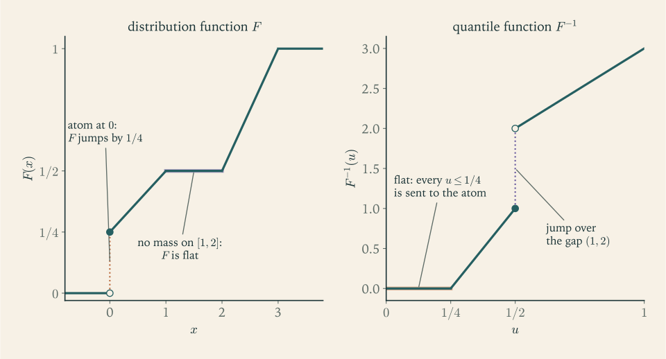
With \(X=F^{-1}(U)\) the mean can be computed on either side:
and, from the law, \(0\cdot\tfrac14+\int_0^1x\cdot\tfrac14\,dx+\int_2^3x\cdot\tfrac12\,dx=\tfrac18+\tfrac54=\tfrac{11}{8}\) . That the two computations must agree is the content of the next section.
1.3 Expectation and the change of variables
Definition 1.10 (expectation). For a random variable \(X\ge 0\) , the expectation is the Lebesgue integral \(\mathbb E X=\int_\Omega X\,d\mathbb P\in[0,\infty]\) . A random variable \(X\) is integrable if \(\mathbb E\lvert X\rvert<\infty\) , and then \(\mathbb E X=\mathbb E X^{+}-\mathbb E X^{-}\) . More generally \(\mathbb E X\) is defined whenever at least one of \(\mathbb E X^{+}\) and \(\mathbb E X^{-}\) is finite. For \(p>0\) , \(L^p\) denotes the set of random variables with \(\mathbb E\lvert X\rvert^p<\infty\) .
Linearity, monotonicity, and the convergence theorems for \(\mathbb E\)
are those of the Lebesgue integral. The definition integrates over \(\Omega\)
, which is rarely where one wants to compute. The following theorem moves every expectation to the space of values. Its proof uses the Monotone Convergence Theorem of Measure Theory: if measurable functions \(h_n\ge 0\)
increase pointwise to \(h\)
, then \(\int h_n\,d\mu\)
increases to \(\int h\,d\mu\)
(math.measure-theory.monotone-convergence-theorem).
Theorem 1.11 (change of variables). Let \(X\) be a random element of \((S,\mathcal S)\) with law \(\mu=\mathbb P_X\) , and let \(h:S\to\mathbb R\) be measurable. If \(h\ge 0\) , then
where both sides may be \(+\infty\) . For general \(h\) , the random variable \(h(X)\) is integrable if and only if \(h\) is \(\mu\) -integrable, and then the same identity holds.
Proof. We climb the standard ladder. For \(h=\mathbf 1_B\) with \(B\in\mathcal S\) , the left side is \(\mathbb P(X\in B)\) and the right side is \(\mu(B)\) ; these agree by the definition of the law. Both sides are linear in \(h\) , so the identity holds for nonnegative simple \(h\) . For measurable \(h\ge 0\) , take simple functions \(0\le h_n\uparrow h\) . Then \(h_n(X)\uparrow h(X)\) on \(\Omega\) , and the Monotone Convergence Theorem, applied once on \((\Omega,\mathcal F,\mathbb P)\) and once on \((S,\mathcal S,\mu)\) , gives
For general \(h\) , apply the nonnegative case to \(\lvert h\rvert\) to see that \(\mathbb E\lvert h(X)\rvert=\int\lvert h\rvert\,d\mu\) , which proves the statement about integrability, and then apply it to \(h^{+}\) and \(h^{-}\) and subtract.
Two special cases are the formulas of a first course. If \(\mu\)
is concentrated on a countable set with \(\mu\{x\}=p(x)\)
, the integral is the sum \(\sum_x h(x)p(x)\)
. If \(\mu\)
has a density \(f\)
with respect to Lebesgue measure, the integral is \(\int h(x)f(x)\,dx\)
. In Probability Theory these two formulas are definitions, and the rule for the density of a transformed variable is a separate technique (math.probability-theory.density-transformation). Here both are corollaries of one identity that holds for every law, including laws that are neither discrete nor given by a density.
Example 1.4: One expectation computed in three places
Let \(X=-\log U\) as in Example 1.2, and compute \(\mathbb E\,e^{-X}\) .
On the sample space, \(e^{-X}=U\) , so the expectation is \(\int_0^1\omega\,d\omega=1/2\) .
On the space of values of \(X\) , the law of \(X\) has density \(e^{-x}\) on \((0,\infty)\) , and Theorem 1.11 with \(h(x)=e^{-x}\) gives \(\int_0^\infty e^{-x}e^{-x}\,dx=1/2\) .
On the space of values of \(W=e^{-X}\) , the law of \(W\) is uniform on \((0,1)\) , and Theorem 1.11 with the identity function gives \(\int_0^1w\,dw=1/2\) .
The same check for the mean of \(X\) reads \(\int_0^1(-\log\omega)\,d\omega=1\) on \(\Omega\) and \(\int_0^\infty xe^{-x}\,dx=1\) on the law. None of the three computations is more correct than the others. The practical content of the theorem is the freedom to choose the easiest.
For nonnegative variables there is a fourth route that needs no density at all. It rests on Tonelli’s theorem from Measure Theory: for a nonnegative measurable function on a product of two sigma-finite measure spaces, the two iterated integrals exist and are equal (math.measure-theory.tonelli-fubini-theorem).
Proposition 1.12 (tail formulas). Let \(Y\ge 0\) be a random variable and \(p>0\) . Then
and
Proof. For each \(\omega\) , \(Y(\omega)^p=\int_0^{\infty}p\,y^{p-1}\mathbf 1_{\{y<Y(\omega)\}}\,dy\) . The integrand is a nonnegative measurable function of \((\omega,y)\) on the product of \((\Omega,\mathcal F,\mathbb P)\) with \(([0,\infty),\mathcal B,\lambda)\) , so Tonelli’s theorem permits taking the expectation inside the integral, which gives the first formula. For the second, the number of integers \(n\ge 1\) with \(n\le Y\) is at most \(Y\) , and the number of integers \(n\ge 0\) with \(n<Y\) is at least \(Y\) ; that is,
Take expectations and exchange expectation and sum, which is legitimate for nonnegative terms by the Monotone Convergence Theorem.
Example 1.5: A censored lifetime
Let \(T\) be exponential with rate \(1\) and let \(X=T\wedge 1\) , a lifetime observed for at most one unit of time. The law of \(X\) has density \(e^{-x}\) on \((0,1)\) and an atom of mass \(\mathbb P(T\ge 1)=e^{-1}\) at the point \(1\) . It is neither discrete nor absolutely continuous, so neither formula of a first course applies as it stands.
The tail formula does not care. Since \(\mathbb P(X>y)=e^{-y}\) for \(0\le y<1\) and \(\mathbb P(X>y)=0\) for \(y\ge 1\) ,
Theorem 1.11 gives the same mean by integrating against both parts of the law: \(\int_0^1xe^{-x}\,dx+1\cdot e^{-1}=(1-2e^{-1})+e^{-1}\) . The variance is \(\mathbb E X^2-(\mathbb E X)^2=1-2e^{-1}-e^{-2}\approx 0.129\) .
1.4 Four inequalities
Proposition 1.13 (Markov and Chebyshev). For a random variable \(X\) and real numbers \(a>0\) , \(p>0\) ,
In particular, if \(X\in L^2\) then \(\mathbb P(\lvert X-\mathbb E X\rvert\ge a)\le\operatorname{Var}(X)/a^2\) .
Proof. Pointwise, \(a^p\mathbf 1_{\{\lvert X\rvert\ge a\}}\le\lvert X\rvert^p\) . Take expectations. The second statement is the first with \(p=2\) applied to \(X-\mathbb E X\) .
Markov’s inequality converts a bound on an average into a bound on a probability, and it is the bridge by which convergence of moments will imply convergence in probability in Chapter 4. The next inequality goes the other way round in spirit: it compares the value of a convex function at an average with the average of its values.
Theorem 1.14 (Jensen’s inequality). Let \(I\subseteq\mathbb R\) be an interval, let \(\varphi:I\to\mathbb R\) be convex, and let \(X\) be an integrable random variable with \(\mathbb P(X\in I)=1\) . Then \(\mathbb E X\in I\) , the expectation \(\mathbb E\,\varphi(X)\) is defined in \((-\infty,\infty]\) , and
Proof. Put \(m=\mathbb E X\) . If \(b\) is the right endpoint of \(I\) , then \(b-X\ge 0\) almost surely, so \(b-m\ge 0\) , and \(b-m=0\) forces \(X=b\) almost surely, in which case \(b\in I\) . The same argument at the left endpoint shows \(m\in I\) , and that if \(m\) is an endpoint then \(X=m\) almost surely and the inequality is an equality.
Suppose then that \(m\) is an interior point of \(I\) . A convex function has a supporting line at each interior point of its domain: there is a real number \(c\) , any number between the left and right derivatives of \(\varphi\) at \(m\) , with
Substituting \(X\) shows that \(\varphi(X)\) is bounded below by an integrable random variable, so \(\mathbb E\,\varphi(X)^{-}<\infty\) and the expectation is defined. Taking expectations gives \(\mathbb E\,\varphi(X)\ge\varphi(m)+c\,(\mathbb E X-m)=\varphi(m)\) .
The inequalities of Hölder and Minkowski are proved in Measure Theory for an arbitrary measure space (math.measure-theory.holder-minkowski): for conjugate exponents \(1<p,q<\infty\)
with \(1/p+1/q=1\)
, \(\mathbb E\lvert XY\rvert\le\lVert X\rVert_p\lVert Y\rVert_q\)
, and for \(p\ge 1\)
, \(\lVert X+Y\rVert_p\le\lVert X\rVert_p+\lVert Y\rVert_p\)
. The case \(p=q=2\)
of the first is the Cauchy–Schwarz inequality. A probability space adds a feature that general measure spaces lack: the \(L^p\)
spaces are nested.
Corollary 1.15 (Lyapunov’s inequality). If \(0<p\le q<\infty\) , then \(\lVert X\rVert_p\le\lVert X\rVert_q\) for every random variable \(X\) . Hence \(L^q\subseteq L^p\) .
Proof. If \(\lVert X\rVert_q=\infty\) there is nothing to prove. Otherwise let \(Y=\lvert X\rvert^p\wedge n\) , which is bounded and hence integrable, and apply Jensen’s inequality to \(Y\) with the convex function \(\varphi(y)=y^{q/p}\) on \([0,\infty)\) : \((\mathbb E\,Y)^{q/p}\le\mathbb E\,Y^{q/p}\le\mathbb E\lvert X\rvert^q\) . Let \(n\to\infty\) and use the Monotone Convergence Theorem on the left, then take \(q\) -th roots.
The total mass being \(1\) is essential. On the real line with Lebesgue measure the constant function \(1\) is bounded and belongs to no \(L^p\) with \(p<\infty\) , and neither of \(L^1(\lambda)\) , \(L^2(\lambda)\) contains the other.
Example 1.6: Expectations that are infinite, and one that is undefined
On \(((0,1),\mathcal B,\lambda)\) with \(U(\omega)=\omega\) , three variables show the three ways an expectation can fail to be an ordinary number or can barely succeed.
The variable \(Z=U^{-1/2}\) . Here \(\mathbb E Z=\int_0^1u^{-1/2}\,du=2\) , while \(\mathbb E Z^2=\int_0^1u^{-1}\,du=\infty\) . So \(Z\in L^1\) and \(Z\notin L^2\) : the inclusion \(L^2\subseteq L^1\) of Corollary 1.15 is strict.
The variable \(Y=1/U\) . Now \(\mathbb E Y=\int_0^1u^{-1}\,du=\infty\) . The expectation is defined, because \(Y\ge 0\) , and it is infinite. The tail formula sees this at once: \(\mathbb P(Y>y)=1/y\) for \(y\ge 1\) , which is not integrable at infinity.
A Cauchy variable. Let \(C=\tan(\pi(U-\tfrac12))\) , which by Theorem 1.9 has the distribution function \(\tfrac12+\tfrac1\pi\arctan x\) and hence the density \(1/(\pi(1+x^2))\) . Then
and by symmetry \(\mathbb E\,C^{-}=\infty\) as well. Both parts are infinite, so \(\mathbb E\,C\) is undefined. The symmetric limit \(\lim_{M\to\infty}\int_{-M}^{M}x/(\pi(1+x^2))\,dx=0\) exists, but it is not an expectation: truncating asymmetrically, at \(-M\) and \(2M\) , gives the limit \(\log 2/\pi\approx 0.221\) instead. Chapter 8 shows that this is no technicality. Averages of independent Cauchy variables do not settle down to \(0\) or to anything else.
Common mistake. Treating equality in law as if it were equality of random variables. From \(V\overset{d}{=}U\) one may not conclude \(U-V=0\) , nor \(\operatorname{Var}(U-V)=0\) , nor \(\mathbb E[UV]=\mathbb E[U^2]\) . In Example 1.2, \(\operatorname{Var}(U-V)=1/3\) , and \(\mathbb E[UV]=\int_0^1u(1-u)\,du=1/6\) while \(\mathbb E[U^2]=1/3\) . Equality in law licenses replacing \(X\) by \(Y\) inside any expression that involves \(X\) alone, such as \(\mathbb E\,h(X)\) . It says nothing about an expression in which \(X\) appears together with another random variable. Before substituting, ask whether the quantity being computed is a functional of one law or of a joint law.
1.5 What the sample space is for
If every question about a random variable can be answered from its law, and every law on the line can be realized on the unit interval, one may fairly ask why the sample space is kept at all. The answer is that probability is rarely about one random variable.
For two random variables \(X\) and \(Y\) on the same space, the pair \((X,Y)\) is a random vector, and its law, a measure on \(\mathbb R^2\) , is called their joint law. The laws of \(X\) and of \(Y\) separately, the marginal laws, are images of the joint law under the coordinate projections, but the joint law is not determined by them: \((U,U)\) and \((U,1-U)\) have the same marginals and live on different diagonals of the unit square. Everything that relates \(X\) to \(Y\) , their covariance, the law of their sum, the probability that one exceeds the other, is a functional of the joint law. A choice of joint law with given marginals is called a coupling, and the sample space is the device that holds a coupling in place.
The need becomes sharper with infinitely many variables. The statement that a sequence \(X_1,X_2,\dots\) converges at \(\omega\) involves all the \(X_n\) at once. Its probability is a functional of the law of the whole sequence, regarded as a random element of the space \(\mathbb R^{\mathbb N}\) with its product sigma-algebra, and it cannot be computed from the laws of the individual \(X_n\) , nor even from the joint laws of all pairs. Chapter 4 exhibits two sequences with identical individual laws of which one converges almost surely and the other does not (Example 4.4), and two sequences in which every pair of terms has the same joint law, with the same contrast (Exercise 4.19).
So the sample space earns its place by carrying joint structure. The first and most important kind of joint structure is the absence of any relation at all, and that is the subject of the next chapter: how is independence expressed for sigma-algebras, with no densities and no product formulas for point masses to lean on, and how does one know that independent sequences with prescribed laws exist?
Exercises
-
Let \(\Omega=\{1,2,3,4\}\) with all subsets as events and let \(X(\omega)=(\omega-2)^2\) . List every event in \(\sigma(X)\) , and decide which of the random variables \(\omega\) , \(\lvert\omega-2\rvert\) , and \(\mathbf 1_{\{2\}}(\omega)\) are \(\sigma(X)\) -measurable, exhibiting the function \(g\) of Theorem 1.5 where one exists.
Answer
The values are \(X(1)=1\) , \(X(2)=0\) , \(X(3)=1\) , \(X(4)=4\) , so the level sets are \(\{2\}\) , \(\{1,3\}\) , \(\{4\}\) and \(\sigma(X)\) consists of the \(8\) unions: \(\emptyset\) , \(\{2\}\) , \(\{4\}\) , \(\{1,3\}\) , \(\{2,4\}\) , \(\{1,2,3\}\) , \(\{1,3,4\}\) , \(\Omega\) . The identity \(\omega\) is not \(\sigma(X)\) -measurable because it separates \(1\) from \(3\) . The variable \(\lvert\omega-2\rvert\) is, with \(g(x)=\sqrt x\) , and so is \(\mathbf 1_{\{2\}}\) , with \(g=\mathbf 1_{\{0\}}\) .
-
Let \(X\) be a random variable. Prove directly from Lemma 1.3 that \(X\) is measurable as soon as \(\{X<q\}\in\mathcal F\) for every rational \(q\) .
Solution
Let \(\mathcal C=\{(-\infty,q):q\in\mathbb Q\}\) . Each member of \(\mathcal C\) is a Borel set, so \(\sigma(\mathcal C)\subseteq\mathcal B(\mathbb R)\) . Conversely, fix a real \(x\) and choose rationals \(q_n>x\) decreasing to \(x\) . Then
\[ (-\infty,x]=\bigcap_{n\ge 1}(-\infty,q_n)\in\sigma(\mathcal C), \]because a point \(y\) lies in every \((-\infty,q_n)\) exactly when \(y\le\lim q_n=x\) . The closed half-lines generate \(\mathcal B(\mathbb R)\) , so \(\mathcal B(\mathbb R)\subseteq\sigma(\mathcal C)\) and the two sigma-algebras coincide. By hypothesis \(X^{-1}(C)=\{X<q\}\in\mathcal F\) for each \(C=(-\infty,q)\in\mathcal C\) , and Lemma 1.3 with this \(\mathcal C\) gives that \(X\) is a random variable.
-
Let \(U\) be uniform on \((0,1)\) . Find the distribution function and a density of \(W=U(1-U)\) , and compute \(\mathbb E\,W\) both from that density and directly on the sample space.
Solution
The function \(u\mapsto u(1-u)\) maps \((0,1)\) onto \((0,1/4]\) and, for \(0<w\le 1/4\) , the inequality \(u(1-u)\le w\) holds exactly when \(u\) lies outside the open interval between the roots \(\tfrac12(1\pm\sqrt{1-4w})\) of \(u^2-u+w\) . That excluded interval has length \(\sqrt{1-4w}\) , so
\[ F_W(w)=1-\sqrt{1-4w},\qquad 0\le w\le\tfrac14 , \]with \(F_W=0\) to the left and \(F_W=1\) to the right. Differentiating, the density is \(f_W(w)=2(1-4w)^{-1/2}\) on \((0,1/4)\) ; it is unbounded near \(1/4\) , where the parabola is flat. From the density, substituting \(s=1-4w\) ,
\[ \mathbb E\,W=\int_0^{1/4}\frac{2w}{\sqrt{1-4w}}\,dw=\frac18\int_0^1\bigl(s^{-1/2}-s^{1/2}\bigr)\,ds=\frac18\Bigl(2-\frac23\Bigr)=\frac16 . \]On the sample space, \(\mathbb E\,W=\int_0^1u(1-u)\,du=\tfrac12-\tfrac13=\tfrac16\) , in agreement with Theorem 1.11.
-
Prove that the distribution function of a random variable has at most countably many points of discontinuity.
Solution
A nondecreasing function has one-sided limits at every point, so \(F\) is discontinuous at \(x\) exactly when the jump \(F(x)-F(x-)\) is positive. For \(n\ge 1\) let \(D_n\) be the set of points at which the jump is at least \(1/n\) . If \(x_1<x_2<\dots<x_k\) are points of \(D_n\) , then the intervals \((F(x_j-),F(x_j)]\) are disjoint subintervals of \([0,1]\) , because \(F(x_j)\le F(x_{j+1}-)\) by monotonicity. Their total length is at least \(k/n\) and at most \(1\) , so \(k\le n\) . Hence each \(D_n\) is finite, with at most \(n\) points, and the set of all discontinuities is the countable union \(\bigcup_nD_n\) of finite sets. In probabilistic terms: a law has at most \(n\) atoms of mass at least \(1/n\) .
-
Let \(X\) and \(Y\) be random variables on the same space with \(X=Y\) almost surely. Prove that \(X\overset{d}{=}Y\) , and give an example on a two-point sample space in which \(X\overset{d}{=}Y\) and \(\mathbb P(X=Y)=0\) .
Solution
Suppose \(\mathbb P(X=Y)=1\) and let \(B\) be a Borel set. The events \(\{X\in B\}\) and \(\{Y\in B\}\) can differ only at points where \(X\ne Y\) , so their symmetric difference is contained in the null event \(\{X\ne Y\}\) . Therefore \(\mathbb P(X\in B)=\mathbb P(Y\in B)\) for every \(B\) , which is \(X\overset{d}{=}Y\) .
For the example take \(\Omega=\{a,b\}\) with \(\mathbb P\{a\}=\mathbb P\{b\}=1/2\) , \(X=\mathbf 1_{\{a\}}\) and \(Y=\mathbf 1_{\{b\}}\) . Each takes the values \(0\) and \(1\) with probability \(1/2\) , so they have the same law, yet \(X(\omega)\ne Y(\omega)\) at both sample points and \(\mathbb P(X=Y)=0\) . This is the two-point version of the pair \(U\) , \(1-U\) .
-
Compute the quantile function of the distribution function \(F(x)=0\) for \(x<1\) , \(F(x)=1-x^{-2}\) for \(x\ge 1\) , and use \(\int_0^1F^{-1}(u)\,du\) to find the mean of the corresponding law.
Solution
For \(0<u<1\) the inequality \(F(x)\ge u\) requires \(x\ge 1\) and \(1-x^{-2}\ge u\) , that is, \(x\ge(1-u)^{-1/2}\) . Since \((1-u)^{-1/2}\ge 1\) , the least such \(x\) is
\[ F^{-1}(u)=(1-u)^{-1/2} . \]By Theorem 1.9 the variable \(X=F^{-1}(U)\) has distribution function \(F\) , and by Theorem 1.11 its mean is the integral of \(F^{-1}\) against Lebesgue measure on \((0,1)\) :
\[ \mathbb E X=\int_0^1(1-u)^{-1/2}\,du=\Bigl[-2(1-u)^{1/2}\Bigr]_0^1=2 . \]As a check from the law itself, \(F\) has density \(2x^{-3}\) on \((1,\infty)\) and \(\int_1^\infty x\cdot 2x^{-3}\,dx=2\) . The second moment is infinite, since \(\int_0^1(1-u)^{-1}\,du\) diverges.
-
Let \(F\) be a continuous distribution function and let \(X\) have distribution function \(F\) . Prove that \(F(X)\) is uniformly distributed on \((0,1)\) , and show by an example with an atom that continuity cannot be dropped.
Solution
Fix \(u\in(0,1)\) and put \(x_u=F^{-1}(u)\) . By Theorem 1.9, \(F(x_u)\ge u\) , and \(F(x)<u\) for every \(x<x_u\) ; letting \(x\uparrow x_u\) and using continuity of \(F\) gives \(F(x_u)\le u\) . So \(F(x_u)=u\) . Again by Theorem 1.9, for any real \(x\) we have \(u\le F(x)\) if and only if \(x_u\le x\) . Applying this with \(x=X(\omega)\) ,
\[ \{F(X)<u\}=\{X<x_u\},\qquad\text{so}\qquad \mathbb P(F(X)<u)=F(x_u-)=F(x_u)=u, \]where continuity is used once more to replace the left limit by the value. Thus \(\mathbb P(F(X)<u)=u\) for all \(u\in(0,1)\) , and letting \(v\downarrow u\) in \(\mathbb P(F(X)<v)=v\) gives \(\mathbb P(F(X)\le u)=u\) . This is the distribution function of the uniform law.
Continuity is needed: if \(X\) takes the values \(0\) and \(1\) with probability \(1/2\) each, then \(F(X)\) takes only the values \(1/2\) and \(1\) , and is not uniform.
-
Let \(F\) and \(F^{-1}\) be as in Theorem 1.9. Prove that \(F(F^{-1}(u))\ge u\) for all \(u\in(0,1)\) and \(F^{-1}(F(x))\le x\) for all \(x\) with \(0<F(x)<1\) , and give an example in which both inequalities are strict.
Solution
The first inequality was established inside the proof of Theorem 1.9: the set \(\{x:F(x)\ge u\}\) is the closed half-line \([F^{-1}(u),\infty)\) , so its left endpoint belongs to it, which says \(F(F^{-1}(u))\ge u\) . For the second, let \(x\) satisfy \(0<F(x)<1\) and put \(u=F(x)\) . The equivalence of Theorem 1.9 reads \(F^{-1}(u)\le x\) if and only if \(u\le F(x)\) ; the right side holds with equality, so \(F^{-1}(F(x))\le x\) .
Both can be strict, and the distribution function of Example 1.3 shows it. Take \(u=1/8\) : then \(F^{-1}(1/8)=0\) and \(F(0)=1/4>1/8\) , the strictness coming from the atom. Take \(x=3/2\) : then \(F(3/2)=1/2\) and \(F^{-1}(1/2)=1<3/2\) , the strictness coming from the flat stretch. Where \(F\) is continuous and strictly increasing, both inequalities are equalities and \(F^{-1}\) is the ordinary inverse.
-
Let \(N\) be a random variable with values in \(\{0,1,2,\dots\}\) . Prove that \(\mathbb E N=\sum_{n\ge 1}\mathbb P(N\ge n)\) , and use it to find the mean of a geometric variable with \(\mathbb P(N\ge n)=(1-p)^{n}\) for \(n\ge 0\) .
Answer
For integer-valued \(N\ge 0\) , \(N=\sum_{n\ge 1}\mathbf 1_{\{N\ge n\}}\) exactly, so both inequalities in the sum form of Proposition 1.12 are equalities. For the geometric variable, \(\mathbb E N=\sum_{n\ge 1}(1-p)^n=(1-p)/p\) .
-
Let \(T\) be exponential with rate \(1\) and \(c>0\) . Use Proposition 1.12 to compute \(\mathbb E[(T\wedge c)^2]\) , and verify that it tends to \(\mathbb E\,T^2=2\) as \(c\to\infty\) , naming the convergence theorem that guarantees this.
Answer
\(\mathbb E[(T\wedge c)^2]=\int_0^c2y\,e^{-y}\,dy=2-2(1+c)e^{-c}\) , which increases to \(2\) . The limit is guaranteed by the Monotone Convergence Theorem, since \((T\wedge c)^2\uparrow T^2\) as \(c\uparrow\infty\) .
-
Prove the one-sided Chebyshev inequality: if \(\mathbb E X=0\) and \(\operatorname{Var}(X)=\sigma^2<\infty\) , then \(\mathbb P(X\ge a)\le\sigma^2/(\sigma^2+a^2)\) for every \(a>0\) . Start from \(\mathbb P(X\ge a)\le\mathbb E[(X+c)^2]/(a+c)^2\) for \(c>0\) and optimize over \(c\) .
Solution
Fix \(c>0\) . On the event \(\{X\ge a\}\) we have \(X+c\ge a+c>0\) , hence \((X+c)^2\ge(a+c)^2\) . Markov’s inequality applied to the nonnegative variable \((X+c)^2\) gives
\[ \mathbb P(X\ge a)\le\frac{\mathbb E(X+c)^2}{(a+c)^2}=\frac{\sigma^2+c^2}{(a+c)^2}, \]using \(\mathbb E X=0\) to expand the square. Call the right side \(r(c)\) . Its derivative has the sign of \(2c(a+c)-2(\sigma^2+c^2)=2(ac-\sigma^2)\) , so \(r\) decreases up to \(c=\sigma^2/a\) and increases afterwards. At the minimizer,
\[ r\!\left(\frac{\sigma^2}{a}\right)=\frac{\sigma^2+\sigma^4/a^2}{(a+\sigma^2/a)^2}=\frac{\sigma^2(a^2+\sigma^2)/a^2}{(a^2+\sigma^2)^2/a^2}=\frac{\sigma^2}{\sigma^2+a^2}. \]The bound is always less than \(1\) , unlike the two-sided bound \(\sigma^2/a^2\) , which is useless for \(a\le\sigma\) .
-
Show that Markov’s inequality is sharp: for given \(a>0\) and \(0<m\le a\) , construct a nonnegative random variable with mean \(m\) and \(\mathbb P(X\ge a)=m/a\) .
Answer
Let \(X=a\) with probability \(m/a\) and \(X=0\) otherwise. Then \(\mathbb E X=m\) and \(\mathbb P(X\ge a)=m/a\) , so Markov’s inequality holds with equality.
-
Use Jensen’s inequality to prove that \(\mathbb E\log X\le\log\mathbb E X\) for an integrable random variable \(X>0\) , and deduce the inequality between the arithmetic and geometric means of positive numbers \(x_1,\dots,x_n\) .
Hint
Apply Theorem 1.14 to the convex function \(\varphi(x)=-\log x\) on \((0,\infty)\) ; the theorem allows \(\mathbb E\,\varphi(X)=+\infty\) . For the means, let \(X\) take each value \(x_i\) with probability \(1/n\) and exponentiate.
-
Let \(X\ge 0\) be a random variable with \(0<\mathbb E X^2<\infty\) . Prove the Paley–Zygmund inequality \(\mathbb P(X>\theta\,\mathbb E X)\ge(1-\theta)^2(\mathbb E X)^2/\mathbb E X^2\) for \(0\le\theta<1\) by applying the Cauchy–Schwarz inequality to \(X\mathbf 1_{\{X>\theta\mathbb E X\}}\) .
Solution
Write \(m=\mathbb E X\) and \(A=\{X>\theta m\}\) . Split the mean according to \(A\) :
\[ m=\mathbb E[X;A^{c}]+\mathbb E[X;A]\le\theta m+\mathbb E[X\mathbf 1_A], \]because \(X\le\theta m\) on \(A^{c}\) . The Cauchy–Schwarz inequality bounds the last term: \(\mathbb E[X\mathbf 1_A]\le(\mathbb E X^2)^{1/2}(\mathbb E\mathbf 1_A^2)^{1/2}=(\mathbb E X^2)^{1/2}\,\mathbb P(A)^{1/2}\) . Hence \((1-\theta)m\le(\mathbb E X^2)^{1/2}\mathbb P(A)^{1/2}\) . Both sides are nonnegative because \(\theta<1\) and \(m\ge 0\) , so squaring preserves the inequality, and dividing by \(\mathbb E X^2>0\) gives
\[ \mathbb P(X>\theta\,\mathbb E X)\ge\frac{(1-\theta)^2(\mathbb E X)^2}{\mathbb E X^2}. \]Where Markov’s inequality bounds the probability of being large from above using one moment, this bounds the probability of not being small from below using two.
-
A student argues: “The variables \(U\) and \(1-U\) have the same law, so \(U+(1-U)\) has the same law as \(U+U\) ; hence the constant \(1\) has the law of \(2U\) .” Identify the invalid step precisely and state what equality in law does allow one to conclude about \(U+(1-U)\) .
Solution
The invalid step is the replacement of \(1-U\) by \(U\) inside the sum \(U+(1-U)\) . That sum is a function of the pair \((U,1-U)\) , and its law is determined by the joint law of the pair, which is concentrated on the line \(\{(x,y):x+y=1\}\) . The sum \(U+U\) is a function of the pair \((U,U)\) , whose joint law is concentrated on the line \(\{x=y\}\) . The two pairs have the same marginal laws and different joint laws, so nothing connects the laws of the two sums; indeed one sum is the constant \(1\) and the other is uniform on \((0,2)\) . Equality in law of \(1-U\) and \(U\) allows the conclusion that \(h(1-U)\overset{d}{=}h(U)\) for every measurable function \(h\) of one variable, for instance that \((1-U)^2\) and \(U^2\) have the same law. About \(U+(1-U)\) it allows no conclusion beyond what direct computation gives.
-
Let \(X\) be a random variable with \(\mathbb E\lvert X\rvert^p<\infty\) for some \(p>0\) . Prove that \(y^p\,\mathbb P(\lvert X\rvert>y)\to 0\) as \(y\to\infty\) , and give an example showing that \(y\,\mathbb P(\lvert X\rvert>y)\to 0\) does not imply \(\mathbb E\lvert X\rvert<\infty\) .
Solution
On the event \(\{\lvert X\rvert>y\}\) we have \(y^p<\lvert X\rvert^p\) , so
\[ y^p\,\mathbb P(\lvert X\rvert>y)\le\mathbb E\bigl[\lvert X\rvert^p;\lvert X\rvert>y\bigr]. \]As \(y\to\infty\) the integrand \(\lvert X\rvert^p\mathbf 1_{\{\lvert X\rvert>y\}}\) tends to \(0\) at every \(\omega\) , since \(\lvert X(\omega)\rvert\) is finite, and it is dominated by the integrable variable \(\lvert X\rvert^p\) . The Dominated Convergence Theorem gives that the right side tends to \(0\) .
For the example, let \(X\ge e\) have the tail \(\mathbb P(X>y)=e/(y\log y)\) for \(y\ge e\) ; this is a legitimate tail, being continuous, decreasing, equal to \(1\) at \(y=e\) , and tending to \(0\) . Then \(y\,\mathbb P(X>y)=e/\log y\to 0\) , while by the tail formula
\[ \mathbb E X=e+\int_e^\infty\frac{e}{y\log y}\,dy=e+e\,\bigl[\log\log y\bigr]_e^\infty=\infty . \] -
For which real \(\alpha\) is \(U^{-\alpha}\) in \(L^p\) , where \(U\) is uniform on \((0,1)\) and \(p>0\) is given? Use the answer to produce, for each pair \(0<p<q\) , a random variable in \(L^p\) that is not in \(L^q\) .
Answer
\(\mathbb E\,U^{-\alpha p}=\int_0^1u^{-\alpha p}\,du\) is finite exactly when \(\alpha p<1\) . Given \(0<p<q\) , the variable \(U^{-1/q}\) is in \(L^p\) , since \(p/q<1\) , and not in \(L^q\) .
-
Let \(X\) be a random element of \((S,\mathcal S)\) and \(h:S\to T\) a measurable map into a second measurable space. Prove that the law of \(h(X)\) is the image of the law of \(X\) under \(h\) , and deduce Theorem 1.11 for a composite \(g(h(X))\) in two different ways.
Hint
For the first part compute \(\{h(X)\in C\}=\{X\in h^{-1}(C)\}\) . For the second, apply Theorem 1.11 once to the random element \(X\) with the function \(g\circ h\) , and once to the random element \(h(X)\) with the function \(g\) ; the first part says the two right-hand sides are integrals of \(g\circ h\) against \(\mathbb P_X\) and of \(g\) against its image under \(h\) .