The oldest theorem of probability says that the average of many independent observations is close to their common mean. Probability Theory states it in its weak form: for independent identically distributed variables with finite variance, the probability that the average of the first \(n\) differs from the mean by more than a given amount tends to zero (math.probability-theory.weak-law-large-numbers). The proof is one application of Chebyshev’s inequality, and it leaves three questions that a first course cannot answer.

Is the variance needed? The statement mentions only the mean, and one suspects that the mean is all that should matter. Is the conclusion true of the sequence of averages actually observed? The weak form speaks of each \(n\) separately; it does not exclude that along the realized sequence the average strays far from the mean again and again, as the typewriter sequence strays from zero. And what happens when there is no mean? If \(X_1,X_2,\dots\) are independent Cauchy variables, the average \((X_1+\dots+X_n)/n\) has exactly the Cauchy law again, for every \(n\) : averaging a million observations is no better than keeping one.

This chapter owns the proofs. It proves the weak law under a first moment only, then the strong law, almost sure convergence of the averages, under the same hypothesis and with independence weakened to pairwise independence, and finally the converse: for independent identically distributed variables the averages converge almost surely to a finite limit if and only if the mean exists. Throughout, \(S_n=X_1+\dots+X_n\) .

8.1 Second moments and a rate

Neither independence nor identical distribution was used, only the additivity of variance. The theorem comes with a rate, and the rate is its limitation: the bound \(C/(n\varepsilon^2)\) is not summable in \(n\) , so the first Borel–Cantelli lemma cannot convert it into almost sure convergence.

8.2 Fourth moments and almost sure convergence

A stronger moment assumption gives a summable bound, and with it the strong law, in a few lines.

The fourth moment grows like \(n^2\) , not \(n^4\) , because of the cancellation in the cross terms: that is where independence enters, and it is what makes the tail of \(S_n/n\) of order \(n^{-2}\) .

8.3 First moments: truncation

With only \(\mathbb E\lvert X_1\rvert<\infty\) there is no variance to feed into Chebyshev’s inequality. The remedy is to manufacture one: cut each variable off at a level beyond which it rarely goes, apply second-moment methods to the bounded pieces, and show that the discarded parts do not matter. This device, truncation, turns out to need nothing beyond the mean.

The three steps, in the order “rarely felt, mean nearly right, variance small”, are the template for every truncation argument. The proof of the strong law has the same three steps, with each strengthened from “tends to zero” to “summable”.

8.4 The strong law

The proof, due to Etemadi, needs two lemmas about the truncated variables. Both are stated for a nonnegative variable; the reduction to that case is the first step of the proof.

It is worth recording where each hypothesis was used. Identical distribution entered through Lemma 8.5 and Step 2. Independence entered exactly once, as the additivity of variance in Step 3, and for that pairwise independence is enough, just as it was for the second Borel–Cantelli lemma in Theorem 3.5. Nonnegativity made \(T_m\) monotone, which is what allowed a sparse subsequence to control everything in between; without monotonicity one needs a maximal inequality, such as Kolmogorov’s inequality of Corollary 7.9, to control the fluctuations between consecutive terms of the subsequence, and that route requires full independence. The subsequence had to be geometric: the factor \(i^{-2}\) in Step 3 is what Lemma 8.5 can absorb, and a subsequence such as \(k_n=n^2\) would produce \(i^{-3/2}\) instead (Exercise 17).

The first moment is not only sufficient.

For independent identically distributed variables there is therefore a clean dichotomy, in keeping with the zero-one law: if \(\mathbb E\lvert X_1\rvert<\infty\) the averages converge almost surely, to the mean; if not, they are almost surely unbounded. Here full independence is used, through the second Borel–Cantelli lemma.

Example 8.3: Cauchy averages do not settle

Let \(X_1,X_2,\dots\) be independent with the Cauchy density \(1/(\pi(1+x^2))\) . The family of Cauchy laws with scale \(a>0\) , with density \(a/(\pi(a^2+x^2))\) , is closed under convolution: the sum of independent Cauchy variables with scales \(a\) and \(b\) is Cauchy with scale \(a+b\) . Chapter 9 will make this a one-line computation with characteristic functions; it can also be verified directly from the convolution integral. Consequently \(S_n\) is Cauchy with scale \(n\) , and \(S_n/n\) is Cauchy with scale \(1\) : the average of \(n\) observations has the law of a single observation. In particular

\[ \mathbb P\Bigl(\Bigl\lvert\frac{S_n}{n}\Bigr\rvert>1\Bigr)=1-\frac2\pi\arctan 1=\frac12\qquad\text{for every }n . \]

No law of large numbers holds, in any mode: \(S_n/n\) does not converge in probability to a constant, and by Theorem 8.6, since \(\mathbb E\lvert X_1\rvert=\infty\) (Example 1.6), \(\limsup_n\lvert S_n\rvert/n=\infty\) almost surely. Even the necessary condition for a weak law with centering constants fails: \(n\,\mathbb P(\lvert X_1\rvert>n)=n(1-\tfrac2\pi\arctan n)\to\tfrac2\pi\) , not \(0\) .

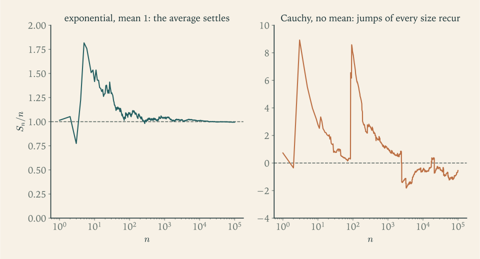
The symmetry of the Cauchy density about \(0\) tempts one to call \(0\) its mean and to expect the averages to approach it. Figure 8.1 shows what happens instead. A single observation of size comparable to \(n\) arrives often enough to move the average by an amount of order \(1\) , at every scale.

8.5 What remains to be said about averages

The strong law is a statement about the limit and is silent about the approach to it. Three kinds of refinement exist, and the rest of the book concerns the first.

Fluctuations. If the variance \(\sigma^2\) is finite, Theorem 8.1 shows that \(S_n/n-\mu\) is of order \(n^{-1/2}\) in mean square. Multiplying by \(\sqrt n\) gives a quantity with constant variance \(\sigma^2\) , and one may ask whether its law settles down. It does, and the limit is the same for all laws with the same variance; that is the central limit theorem, proved in Chapter 10. The convergence there is only in distribution, the weakest mode of Chapter 4, and it requires a separate theory, which is the subject of Chapter 9.

Almost sure rates. The strong law says \(S_n-n\mu=o(n)\) almost surely. The sharp almost sure statement, for finite variance, is the law of the iterated logarithm, \(\limsup_n(S_n-n\mu)/\sqrt{2\sigma^2n\log\log n}=1\) , which we mention without proof.

Dependence. Independence was used through the additivity of variances and through the Borel–Cantelli lemmas. Sequences in which the variables are dependent can obey laws of large numbers for other reasons, as martingale differences or as stationary sequences do, and they can also fail to: if \(X_n=X_1\) for all \(n\) the averages equal \(X_1\) and converge to a random limit. Such results belong to the study of stochastic processes.

The next chapter develops convergence of laws. Its opening question is one of definition: the constants \(1/n\) surely converge in distribution to \(0\) , and yet their distribution functions do not converge to the distribution function of \(0\) at the origin. What is the right notion?

Exercises

1. Let \(X_1,X_2,\dots\) be pairwise uncorrelated with mean \(\mu\) and variances \(\sigma_k^2\) , not assumed bounded. Show that \(S_n/n\to\mu\) in \(L^2\) if and only if \(n^{-2}\sum_{k\le n}\sigma_k^2\to 0\) , and give an example with \(\sigma_k^2\to\infty\) in which this holds.

   Hint

   \(\mathbb E(S_n/n-\mu)^2=n^{-2}\sum_{k\le n}\sigma_k^2\) exactly, by Corollary 2.7. Example: \(\sigma_k^2=\sqrt k\) , for which \(n^{-2}\sum_{k\le n}\sqrt k\le n^{-1/2}\to 0\) .

2. Let \(X_1,\dots,X_n\) be independent and identically distributed with mean \(0\) , variance \(\sigma^2\) , and fourth moment \(m_4\) . Prove that \(\mathbb E S_n^4=nm_4+3n(n-1)\sigma^4\) , and verify the formula by enumeration for \(n=3\) when \(X\) takes the values \(-1,0,1\) with probabilities \(\tfrac14,\tfrac12,\tfrac14\) .

   Solution

   Expand \(S_n^4=\sum_{i,j,k,l}X_iX_jX_kX_l\) over all \(n^4\) quadruples and take expectations. If some index value occurs exactly once in the quadruple, the corresponding factor is independent of the product of the others and has mean \(0\) , so the term vanishes by Theorem 2.6. The remaining quadruples are of two kinds. Those with all four indices equal number \(n\) , and each contributes \(m_4\) . Those in which two distinct values each occur twice: the unordered pair of values can be chosen in \(\binom n2\) ways, and the two positions occupied by the smaller value in \(\binom42=6\) ways, giving \(6\binom n2=3n(n-1)\) quadruples, each contributing \(\mathbb E X_i^2\,\mathbb E X_j^2=\sigma^4\) . Hence

   \[ \mathbb E S_n^4=n\,m_4+3n(n-1)\,\sigma^4 . \]

   For the three-point law, \(\sigma^2=\mathbb E X^2=\tfrac12\) and \(m_4=\mathbb E X^4=\tfrac12\) , so the formula gives \(\mathbb E S_3^4=\tfrac32+18\cdot\tfrac14=6\) . Enumerating the \(27\) value patterns with their probabilities and averaging \((X_1+X_2+X_3)^4\) also gives \(6\) . The point of the formula is the order of magnitude: \(n^2\) , not \(n^4\) , because only paired indices survive.

3. Let \(X_1,X_2,\dots\) be pairwise uncorrelated with mean \(0\) and \(\lvert X_k\rvert\le K\) . Prove that \(S_n/n\to 0\) almost surely by first treating the subsequence \(n=k^2\) with Theorem 8.1 and then bounding \(\lvert S_n-S_{k^2}\rvert\) for \(k^2\le n<(k+1)^2\) .

   Solution

   Along squares. The variances are at most \(K^2\) , so by Theorem 8.1, \(\mathbb P(\lvert S_{k^2}\rvert\ge\varepsilon k^2)\le K^2/(k^2\varepsilon^2)\) . These bounds are summable in \(k\) , and the first Borel–Cantelli lemma gives \(\lvert S_{k^2}\rvert/k^2<\varepsilon\) for all large \(k\) , almost surely. With \(\varepsilon=1/j\) and an intersection over \(j\) , \(S_{k^2}/k^2\to 0\) almost surely.

   Between squares. For \(k^2\le n<(k+1)^2\) the sum \(S_n-S_{k^2}\) has \(n-k^2\le 2k\) terms, each bounded by \(K\) , so \(\lvert S_n-S_{k^2}\rvert\le 2kK\) at every sample point. Therefore

   \[ \frac{\lvert S_n\rvert}{n}\le\frac{\lvert S_{k^2}\rvert}{k^2}+\frac{2kK}{k^2}\longrightarrow 0\qquad\text{almost surely,} \]

   since \(k\to\infty\) as \(n\to\infty\) . The subsequence \(k^2\) is dense enough that bounded terms cannot move the average between consecutive squares, and sparse enough that Chebyshev’s bound becomes summable. For unbounded variables the gaps are the difficulty, which is why the proof of Theorem 8.4 needs truncation and monotonicity.

4. Let \(f\) be continuous on \([0,1]\) and let \(B_nf(p)=\sum_{k=0}^{n}f(k/n)\binom nkp^k(1-p)^{n-k}\) . Use Theorem 8.1 to prove that \(B_nf\to f\) uniformly on \([0,1]\) , and bound \(\sup_p\lvert B_nf(p)-f(p)\rvert\) for \(f(x)=\lvert x-\tfrac12\rvert\) and \(n=100\) .

   Solution

   Fix \(p\in[0,1]\) and let \(S_n\) be the number of successes in \(n\) independent trials with success probability \(p\) , so that \(B_nf(p)=\mathbb E f(S_n/n)\) . Let \(M=\sup\lvert f\rvert\) and \(\varepsilon>0\) . By uniform continuity of \(f\) on \([0,1]\) there is \(\delta>0\) with \(\lvert f(x)-f(y)\rvert\le\varepsilon\) whenever \(\lvert x-y\rvert\le\delta\) . Splitting according to whether \(\lvert S_n/n-p\rvert\le\delta\) ,

   \[ \lvert B_nf(p)-f(p)\rvert\le\mathbb E\lvert f(S_n/n)-f(p)\rvert\le\varepsilon+2M\,\mathbb P\bigl(\lvert S_n/n-p\rvert>\delta\bigr)\le\varepsilon+\frac{2M\,p(1-p)}{n\delta^2}\le\varepsilon+\frac{M}{2n\delta^2}, \]

   by Theorem 8.1 with variance \(p(1-p)\le\tfrac14\) . The bound does not depend on \(p\) , so \(\limsup_n\sup_p\lvert B_nf(p)-f(p)\rvert\le\varepsilon\) for every \(\varepsilon\) : the convergence is uniform. This is Weierstrass’s approximation theorem, with explicit polynomials.

   For \(f(x)=\lvert x-\tfrac12\rvert\) we have \(M=\tfrac12\) and may take \(\delta=\varepsilon\) , giving the bound \(\varepsilon+1/(4n\varepsilon^2)\) ; with \(n=100\) the best choice \(\varepsilon=200^{-1/3}\approx 0.171\) gives \(0.256\) . The actual maximal error, attained at \(p=\tfrac12\) , is \(\mathbb E\lvert S_{100}/100-\tfrac12\rvert\approx 0.0398\) . As in Example 8.1, the Chebyshev bound proves convergence and overstates the error.

5. Prove that almost every number in \((0,1)\) is normal in base \(10\) in the strong sense that every finite block of digits occurs with its expected frequency, by applying the strong law to suitable indicator variables that are independent along arithmetic progressions.

   Hint

   The decimal digits of a uniform point are independent and uniform on \(\{0,\dots,9\}\) : the proof of Proposition 2.8 applies word for word with intervals of length \(10^{-n}\) in place of \(2^{-n}\) , as Example 2.5 notes for base three. Fix a block \(w\) of length \(r\) . The indicators that the digits in positions \(jr+s+1,\dots,jr+s+r\) equal \(w\) , for \(j=0,1,2,\dots\) and a fixed offset \(s\in\{0,\dots,r-1\}\) , are functions of disjoint groups of digits, hence independent by Corollary 2.4, with mean \(10^{-r}\) . Apply Theorem 8.2 for each offset, average over the \(r\) offsets, and intersect over the countably many blocks.

6. A student writes: “The Cauchy density is symmetric about \(0\) , so by the law of large numbers the average of \(n\) independent Cauchy observations is close to \(0\) for large \(n\) .” Compute \(\mathbb P(\lvert S_n/n\rvert>1)\) , identify the hypothesis that fails, and state what Theorem 8.6 says about these averages.

   Solution

   By Example 8.3 the average \(S_n/n\) has the same Cauchy law as a single observation, for every \(n\) . Its distribution function is \(\tfrac12+\tfrac1\pi\arctan x\) , so

   \[ \mathbb P\Bigl(\Bigl\lvert\frac{S_n}{n}\Bigr\rvert>1\Bigr)=1-\frac2\pi\arctan 1=1-\frac2\pi\cdot\frac\pi4=\frac12\qquad\text{for all }n . \]

   The average is not close to \(0\) for large \(n\) ; it is as dispersed as one observation. The hypothesis that fails is integrability: \(\mathbb E\lvert X_1\rvert=\infty\) (Example 1.6), so the Cauchy law has no mean. Symmetry about \(0\) makes \(0\) the median and the centre of symmetry, and neither of these is what a law of large numbers is about. Theorem 8.6 gives the precise statement: since the observations are independent and identically distributed with \(\mathbb E\lvert X_1\rvert=\infty\) , almost surely \(\limsup_n\lvert S_n\rvert/n=\infty\) . The averages are not merely non-convergent but unbounded along almost every sequence of observations, as in the right panel of Figure 8.1.

7. Let \(X_1,X_2,\dots\) be independent with \(\mathbb P(X_k=2^j)=2^{-j}\) for \(j\ge 1\) . Show that \(\mathbb E X_1=\infty\) and that \(S_n/(n\log_2n)\to 1\) in probability, by truncating at the level \(n\log_2n\) .

   Hint

   \(\mathbb E X_1=\sum_j2^j2^{-j}=\infty\) . With \(b_n=n\log_2n\) and \(X_k'=X_k\mathbf 1_{\{X_k\le b_n\}}\) : \(n\,\mathbb P(X_1>b_n)\le 2n/b_n\to 0\) ; \(\mathbb E X_1'\) is the number of \(j\) with \(2^j\le b_n\) , which is \(\log_2n+\log_2\log_2n+O(1)\) ; and \(\operatorname{Var}(\sum_{k\le n}X_k')\le n\sum_{2^j\le b_n}2^j\le 2nb_n\) , which is small compared with \(b_n^2\) . Conclude as in Theorem 8.3.

8. Let \(X_1,X_2,\dots\) be independent and identically distributed with \(\mathbb E X_1^{+}=\infty\) and \(\mathbb E X_1^{-}<\infty\) . Prove that \(S_n/n\to\infty\) almost surely.

   Solution

   For \(M>0\) let \(X_k^{M}=X_k\wedge M\) . These variables are independent and identically distributed, and integrable: the positive part is at most \(M\) and the negative part equals \(X_k^{-}\) , which is integrable by hypothesis. By Theorem 8.4,

   \[ \liminf_{n\to\infty}\frac{S_n}{n}\ \ge\ \lim_{n\to\infty}\frac1n\sum_{k\le n}X_k^{M}=\mathbb E[X_1\wedge M]\qquad\text{almost surely,} \]

   because \(X_k\ge X_k^{M}\) . This holds for each \(M\) outside a null event, hence for all integers \(M\) simultaneously outside a null event. As \(M\uparrow\infty\) , the variables \(X_1\wedge M+X_1^{-}\) are nonnegative and increase to \(X_1^{+}\) , so by monotone convergence \(\mathbb E[X_1\wedge M]\uparrow\mathbb E X_1^{+}-\mathbb E X_1^{-}=\infty\) . Therefore \(\liminf_nS_n/n=\infty\) almost surely. Truncation from above produced integrable variables whose averages bound the original averages from below; the strong law for the truncated variables did the rest.

9. Let \(X_1,X_2,\dots\) be independent and identically distributed with mean \(\mu>0\) . Show that \(S_n\to\infty\) almost surely and that \(\inf_nS_n>-\infty\) almost surely.

   Answer

   By Theorem 8.4, \(S_n/n\to\mu>0\) almost surely, so almost surely \(S_n>n\mu/2\) for all large \(n\) ; hence \(S_n\to\infty\) , and the infimum over \(n\) is the minimum of finitely many finite values.

10. Let \(\xi_1,\xi_2,\dots\) be independent, identically distributed, and positive with mean \(\mu\in(0,\infty)\) , let \(T_n=\xi_1+\dots+\xi_n\) , and let \(N_t=\max\{n:T_n\le t\}\) . Prove that \(N_t/t\to 1/\mu\) almost surely as \(t\to\infty\) .

    Solution

    Since each \(T_n\) is finite, \(N_t\to\infty\) as \(t\to\infty\) at every sample point, and since \(T_n\to\infty\) almost surely (by the strong law, \(T_n/n\to\mu>0\) ), \(N_t\) is finite for every \(t\) . By the definition of \(N_t\) ,

    \[ T_{N_t}\le t<T_{N_t+1},\qquad\text{so}\qquad\frac{T_{N_t}}{N_t}\le\frac{t}{N_t}<\frac{T_{N_t+1}}{N_t+1}\cdot\frac{N_t+1}{N_t} \]

    once \(N_t\ge 1\) . On the event of probability one where \(T_n/n\to\mu\) , the same limit holds along the integers \(N_t\) and \(N_t+1\) , because they tend to infinity; and \((N_t+1)/N_t\to 1\) . Both outer terms tend to \(\mu\) , so \(t/N_t\to\mu\) , that is, \(N_t/t\to 1/\mu\) almost surely. The argument is purely pathwise once the strong law has been applied: it converts a statement about the time of the \(n\) -th event into a statement about the number of events by time \(t\) . This is the elementary renewal law used in the study of Stochastic Processes.

11. Let \(X_1,X_2,\dots\) be independent with common distribution function \(F\) and let \(F_n(x)=\tfrac1n\sum_{k\le n}\mathbf 1_{\{X_k\le x\}}\) . Show that \(F_n(x)\to F(x)\) almost surely for each \(x\) , and that when \(F\) is continuous the convergence is almost surely uniform in \(x\) .

    Hint

    For fixed \(x\) the indicators \(\mathbf 1_{\{X_k\le x\}}\) are independent and identically distributed with mean \(F(x)\) . For uniformity with \(F\) continuous, choose points \(x_1<\dots<x_m\) with \(F(x_{i+1})-F(x_i)\le\varepsilon\) and use monotonicity of \(F_n\) and \(F\) between them.

12. For \(X\) exponential with rate \(1\) evaluate the two sums in Proposition 1.12 that bracket \(\mathbb E X\) , and evaluate \(\sum_{k\ge 1}\mathbb P(X>k)\) as it appears in Lemma 8.5.

    Answer

    \(\sum_{n\ge 1}\mathbb P(X\ge n)=\sum_{n\ge 1}e^{-n}=1/(e-1)\approx 0.582\) and \(\sum_{n\ge 0}\mathbb P(X>n)=e/(e-1)\approx 1.582\) , which bracket \(\mathbb E X=1\) . In Lemma 8.5, \(\sum_{k\ge 1}\mathbb P(X>k)=1/(e-1)\) .

13. Let \(X_1,X_2,\dots\) be independent and identically distributed and not almost surely \(0\) . Show that the series \(\sum_nX_n\) converges with probability \(0\) .

    Answer

    If the series converged, its terms would tend to \(0\) . But for some \(\varepsilon>0\) , \(\mathbb P(\lvert X_1\rvert>\varepsilon)>0\) , and the independent events \(\{\lvert X_n\rvert>\varepsilon\}\) have this same probability, so by the second Borel–Cantelli lemma they occur infinitely often almost surely.

14. Let \(X\) be symmetric with \(\mathbb P(\lvert X\rvert>x)=e/(x\log x)\) for \(x\ge e\) . Show that \(\mathbb E\lvert X\rvert=\infty\) while \(n\,\mathbb P(\lvert X\rvert>n)\to 0\) , and adapt the proof of Theorem 8.3 to show that \(S_n/n\to 0\) in probability for independent copies; conclude with Theorem 8.6 that the weak law can hold where the strong law fails.

    Hint

    \(\mathbb E\lvert X\rvert=\infty\) by Exercise 1.16, and \(n\,\mathbb P(\lvert X\rvert>n)=e/\log n\to 0\) . In the proof of Theorem 8.3 the first step needs only \(n\,\mathbb P(\lvert X_1\rvert>n)\to 0\) ; the truncated means vanish by symmetry; and \(\tfrac1n\mathbb E[X_1^2;\lvert X_1\rvert\le n]\le\tfrac1n\int_0^n2y\,\mathbb P(\lvert X_1\rvert>y)\,dy\to 0\) as an average of a function tending to \(0\) .

15. Prove the \(L^1\) assertion of Theorem 8.4 in full: explain why \((X_k)\) is uniformly integrable, why the averages are, and which theorem then gives \(\mathbb E\lvert S_n/n-\mu\rvert\to 0\) .

    Solution

    The variables. The \(X_k\) all have the law of \(X_1\) , so for every \(k\) , \(\mathbb E[\lvert X_k\rvert;\lvert X_k\rvert>M]=\mathbb E[\lvert X_1\rvert;\lvert X_1\rvert>M]\) , which tends to \(0\) as \(M\to\infty\) because \(X_1\) is integrable. The supremum over \(k\) of these equal quantities tends to \(0\) : the sequence \((X_k)\) is uniformly integrable. No independence is involved.

    The averages. By Proposition 5.5 the averages \(\bar X_n=S_n/n\) of a uniformly integrable sequence are uniformly integrable; the proof used the two faces of Proposition 5.2 and the bound \(\mathbb E[\lvert\bar X_n\rvert;A]\le\sup_k\mathbb E[\lvert X_k\rvert;A]\) .

    The limit. By the almost sure part of Theorem 8.4, \(\bar X_n\to\mu\) almost surely, hence in probability. The Vitali convergence theorem (Theorem 5.6, from (i) to (ii)) now gives \(\mathbb E\lvert\bar X_n-\mu\rvert\to 0\) . Domination would not have been available: \(\sup_n\lvert\bar X_n\rvert\) need not be integrable when \(X_1\) is merely integrable, so the Dominated Convergence Theorem cannot replace Vitali’s theorem here.

16. An event has unknown probability \(p\) . Use Theorem 8.1 to find a number of independent trials that guarantees, for every \(p\) , that the observed frequency is within \(0.01\) of \(p\) with probability at least \(0.95\) .

    Answer

    The variance of an indicator is \(p(1-p)\le\tfrac14\) , so Theorem 8.1 gives the bound \(1/(4n\cdot 10^{-4})\) , which is at most \(0.05\) when \(n\ge 50{,}000\) .

17. In the proof of Theorem 8.4, say exactly where identical distribution, pairwise independence, and nonnegativity are used. Then repeat Step 3 with the subsequence \(k_n=n^2\) in place of \(\lfloor\alpha^n\rfloor\) and show which series would have to converge, and why Lemma 8.5 does not provide it.

    Solution

    Identical distribution is used three times: in Step 1, to write \(\sum_k\mathbb P(X_k>k)=\sum_k\mathbb P(X_1>k)\) and apply Lemma 8.5; in Step 2, to get \(\mathbb E Y_k=\mathbb E[X_1;X_1\le k]\uparrow\mu\) ; and in Step 3, to write \(\mathbb E Y_i^2=\mathbb E[X_1^2;X_1\le i]\) and apply Lemma 8.5 again. Pairwise independence is used once, in Step 3, for \(\operatorname{Var}(T_m)=\sum_{i\le m}\operatorname{Var}(Y_i)\) ; the \(Y_i\) are pairwise independent as functions of the \(X_i\) . Nonnegativity is used in Step 2 for monotone convergence and, decisively, in Step 4, where it makes \(T_m\) nondecreasing so that \(T_m/m\) can be sandwiched.

    Now take \(k_n=n^2\) . The inner sum in Step 3 becomes

    \[ \sum_{n:\,n^2\ge i}\frac1{n^4}\ \approx\ \int_{\sqrt i}^\infty\frac{dt}{t^4}=\frac{1}{3\,i^{3/2}}, \]

    so the argument would require \(\sum_i\operatorname{Var}(Y_i)\,i^{-3/2}<\infty\) . Lemma 8.5 controls only \(\sum_i\mathbb E Y_i^2\,i^{-2}\) , and the stronger series can diverge: for the law of Example 8.5, \(\mathbb E Y_i^2=3(\sqrt i-1)\) and \(\sum_i\sqrt i\cdot i^{-3/2}=\sum_i1/i=\infty\) . A polynomial subsequence has too many terms below each index \(i\) ; a geometric one has only about \(\log i\) of them, with reciprocal squares summing to order \(i^{-2}\) . The price of a geometric subsequence is large gaps, and the limits \(\mu/\alpha\) and \(\alpha\mu\) in Step 4, with \(\alpha\downarrow 1\) , are how the proof pays it.

18. Kronecker’s lemma states that if \(\sum_ka_k/k\) converges then \(\tfrac1n\sum_{k\le n}a_k\to 0\) . Use it with Theorem 7.15 to prove that independent mean-zero variables with \(\sum_k\operatorname{Var}(X_k)/k^2<\infty\) satisfy \(S_n/n\to 0\) almost surely.

    Hint

    The partial sums \(\sum_{k\le n}X_k/k\) form a martingale with \(\mathbb E(\sum_{k\le n}X_k/k)^2=\sum_{k\le n}\operatorname{Var}(X_k)/k^2\) , bounded by hypothesis; Theorem 7.15 gives almost sure convergence of \(\sum_kX_k/k\) , and Kronecker’s lemma applied pathwise with \(a_k=X_k(\omega)\) gives \(S_n/n\to 0\) .