The strong law says that \(S_n/n-\mu\to 0\) . At what magnification do the fluctuations of the average around the mean become visible, and what do they look like? If the variance \(\sigma^2\) is finite and positive, the variance of \(S_n-n\mu\) is \(n\sigma^2\) , so the standardized sum
has mean \(0\) and variance \(1\) for every \(n\) : the magnification \(\sqrt n\) is exactly right to keep the fluctuations at a fixed scale. The question is whether the law of \(Z_n\) settles down.
A heuristic identifies the only possible limit. Split a sum of \(2n\) terms into two halves. Then \(Z_{2n}=(Z_n+Z_n')/\sqrt2\) , where \(Z_n'\) is an independent copy of \(Z_n\) . If the laws converge to some law with characteristic function \(\psi\) , then \(\psi(t)=\psi(t/\sqrt2)^2\) , and among laws with variance \(1\) this functional equation singles out \(\psi(t)=e^{-t^2/2}\) . The limit, if there is one, is the standard normal law, whatever the law of the individual terms.
The classical statement of this central limit theorem, and its use for approximating probabilities, belong to Probability Theory (math.probability-theory.central-limit-theorem). This chapter owns the proof, which is short now that Chapter 9 is available; the extension to sums of variables that are not identically distributed, with the exact condition under which the normal limit holds; and the caveats about what the theorem does not assert. Its last section looks back over the whole book and asks, for a given question about a given sequence, which limit theorem to reach for.
10.1 The characteristic function near the origin
The proof needs to know how a characteristic function behaves near \(t=0\) when the law has two moments. Everything comes from a careful form of Taylor’s theorem for \(e^{ix}\) .
Lemma 10.1 (Taylor estimate for the complex exponential). For real \(x\) and every integer \(n\ge 0\) ,
Proof. Let \(R_n(x)\) be the difference on the left. For \(n=0\) , \(R_0(x)=e^{ix}-1=i\int_0^xe^{is}\,ds\) , so \(\lvert R_0(x)\rvert\le\min(\lvert x\rvert,2)\) . For \(n\ge 1\) , differentiating shows \(R_n'(x)=iR_{n-1}(x)\) and \(R_n(0)=0\) , so \(R_n(x)=i\int_0^xR_{n-1}(s)\,ds\) and \(\lvert R_n(x)\rvert\le\int_0^{\lvert x\rvert}\lvert R_{n-1}(s)\rvert\,ds\) . By induction, integrating each of the two bounds for \(R_{n-1}\) gives the two bounds for \(R_n\) .
The first bound is the usual one, good for small \(x\) . The second is better for large \(x\) , and its presence is what allows the lemma to be integrated against a law with only \(n\) moments.
Proposition 10.2 (second-order expansion). Let \(X\) have mean \(0\) and finite variance \(\sigma^2\) , and characteristic function \(\varphi\) . Then for all real \(t\) ,
and the expectation on the right tends to \(0\) as \(t\to 0\) . Thus \(\varphi(t)=1-\tfrac12\sigma^2t^2+o(t^2)\) .
Proof. Lemma 10.1 with \(n=2\) and \(x=tX\) gives \(\lvert e^{itX}-1-itX+\tfrac12t^2X^2\rvert\le\min(\lvert tX\rvert^3/6,\,t^2X^2)\) . Take expectations, using \(\mathbb E X=0\) and \(\mathbb E X^2=\sigma^2\) . The integrand \(\min(\lvert t\rvert\lvert X\rvert^3/6,X^2)\) is dominated by the integrable variable \(X^2\) and tends to \(0\) pointwise as \(t\to 0\) , so its expectation tends to \(0\) by dominated convergence.
No third moment was assumed. The cubic bound is used where \(X\) is moderate and the quadratic bound where it is large.
10.2 The Lindeberg–Lévy theorem
Theorem 10.3 (central limit theorem). Let \(X_1,X_2,\dots\) be independent and identically distributed with mean \(\mu\) and variance \(\sigma^2\in(0,\infty)\) . Then
Proof. Replacing \(X_k\) by \((X_k-\mu)/\sigma\) , we may assume \(\mu=0\) and \(\sigma=1\) . Let \(\varphi\) be the common characteristic function. By Proposition 9.11 the characteristic function of \(S_n/\sqrt n\) is \(\varphi(t/\sqrt n)^n\) . Fix \(t\) and put \(c_n=n\bigl(\varphi(t/\sqrt n)-1\bigr)\) . By Proposition 10.2 applied at the point \(t/\sqrt n\) ,
So \(c_n\to-t^2/2\) , and by Lemma 9.16, \(\varphi(t/\sqrt n)^n=(1+c_n/n)^n\to e^{-t^2/2}\) . This is the characteristic function of the standard normal law (Example 9.4). By Lévy’s continuity theorem (Theorem 9.17), \(S_n/\sqrt n\) converges in distribution to that law.
Since the normal distribution function \(\Phi\) is continuous, Theorem 9.2 gives \(\mathbb P(Z_n\le x)\to\Phi(x)\) for every \(x\) . The proof used independence only through the product formula for characteristic functions, identical distribution only to have a single \(\varphi\) , and the variance only through the second-order expansion at the origin. The law of the terms has otherwise disappeared: its characteristic function was evaluated only at points tending to \(0\) , where all laws with mean \(0\) and variance \(1\) agree to second order.
Example 10.1: Two characteristic functions approaching the Gaussian
Random signs. If \(X=\pm1\) with probability \(\tfrac12\) each, then \(\varphi(t)=\cos t\) and the characteristic function of \(S_n/\sqrt n\) is \(\cos(t/\sqrt n)^n\) . At \(t=1\) its values are \(0.6014\) for \(n=10\) and \(0.6060\) for \(n=100\) , against the limit \(e^{-1/2}\approx 0.6065\) . For \(n=1\) it is \(\cos t\) , which returns to \(1\) at \(t=2\pi\) , the mark of a law carried by a lattice; taking \(n\) -th powers at the shrunken argument pushes these returns out to \(t=2\pi\sqrt n\) and flattens everything before them.
Centred exponential variables. If \(X=T-1\) with \(T\) exponential of rate \(1\) , then \(\varphi(t)=e^{-it}/(1-it)\) , which is not real because the law is not symmetric. The characteristic function of \(S_n/\sqrt n\) at \(t=1\) is \(0.6178-0.0617i\) for \(n=10\) and \(0.6077-0.0201i\) for \(n=100\) . The imaginary part, which records the skewness of the sum, decays like \(n^{-1/2}\) ; the modulus is \((1+t^2/n)^{-n/2}\) , which tends to \(e^{-t^2/2}\) .
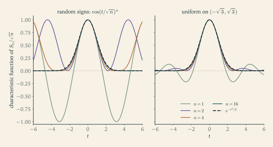
Example 10.2: A binomial probability, three ways
Let \(S_{100}\) be the number of heads in \(100\) fair tosses, with mean \(50\) and standard deviation \(5\) . The exact probability of at most \(55\) heads is the binomial sum \(\mathbb P(S_{100}\le 55)=0.8644\) . Theorem 10.3 suggests \(\Phi((55-50)/5)=\Phi(1)=0.8413\) . The error, \(0.023\) , is not small; it arises because the distribution function of \(S_{100}\) jumps by \(\mathbb P(S_{100}=55)\approx 0.048\) at \(55\) , and a continuous function cannot follow a jump. Evaluating \(\Phi\) halfway to the next atom, at \((55.5-50)/5=1.1\) , gives \(\Phi(1.1)=0.8643\) , which is correct to three decimals. This continuity correction is a matter of numerical practice and is not part of the theorem.
The theorem says that \(\sup_x\lvert\mathbb P(Z_n\le x)-\Phi(x)\rvert\to 0\) (for a continuous limit, pointwise convergence of distribution functions is automatically uniform, a fact due to Pólya that we use only in this remark and do not prove) and gives no rate. Here the supremum is attained at the central atom and equals half its mass, \(0.0398\) . A rate requires a further moment. The Berry–Esseen theorem, which we state without proof, asserts that if \(\rho=\mathbb E\lvert X_1-\mu\rvert^3<\infty\) then
for an absolute constant \(C\) , whose best value is known to lie between \(0.4097\) and \(0.4748\) . For the fair coin \(\rho/\sigma^3=1\) , and with \(C=0.4748\) and \(n=100\) the bound is \(0.0475\) , against the true value \(0.0398\) : the rate \(n^{-1/2}\) cannot be improved in general, and the lattice structure of the coin is what saturates it.
10.3 Sums of unequal terms
Identical distribution is a convenience, not the heart of the matter. The natural setting is a triangular array: for each \(n\) a finite family of independent variables, with no relation required between the families for different \(n\) .
Lemma 10.4 (comparison of products). If \(z_1,\dots,z_m\) and \(w_1,\dots,w_m\) are complex numbers of modulus at most \(1\) , then \(\bigl\lvert\prod_kz_k-\prod_kw_k\bigr\rvert\le\sum_k\lvert z_k-w_k\rvert\) .
Proof. For \(m=1\) there is nothing to prove. For the inductive step write \(\prod_{k\le m}z_k-\prod_{k\le m}w_k=z_m\bigl(\prod_{k<m}z_k-\prod_{k<m}w_k\bigr)+(z_m-w_m)\prod_{k<m}w_k\) and use that \(\lvert z_m\rvert\le 1\) and \(\lvert\prod_{k<m}w_k\rvert\le 1\) .
Theorem 10.5 (Lindeberg–Feller central limit theorem). For each \(n\) let \(X_{n,1},\dots,X_{n,k_n}\) be independent random variables with mean \(0\) and variances \(\sigma_{n,k}^2\) satisfying \(\sum_k\sigma_{n,k}^2=1\) . Suppose that for every \(\varepsilon>0\) ,
Then \(S_n=X_{n,1}+\dots+X_{n,k_n}\) converges in distribution to \(N(0,1)\) .
Proof. Let \(\varphi_{n,k}\) be the characteristic function of \(X_{n,k}\) ; that of \(S_n\) is \(\prod_k\varphi_{n,k}\) . Fix \(t\) .
Step 1: every term is small. For each \(k\) and \(\varepsilon>0\) , \(\sigma_{n,k}^2\le\varepsilon^2+\mathbb E[X_{n,k}^2;\lvert X_{n,k}\rvert>\varepsilon]\le\varepsilon^2+L_n(\varepsilon)\) . Hence \(\max_k\sigma_{n,k}^2\to 0\) . In particular, for large \(n\) the numbers \(a_{n,k}=\tfrac12\sigma_{n,k}^2t^2\) lie in \([0,1]\) .
Step 2: replace each factor by its second-order expansion. By Lemma 10.1 with \(n=2\) , as in Proposition 10.2, and splitting according to whether \(\lvert X_{n,k}\rvert\le\varepsilon\) ,
Both \(\varphi_{n,k}(t)\) and \(1-a_{n,k}\) have modulus at most \(1\) for large \(n\) , so by Lemma 10.4 and \(\sum_k\sigma_{n,k}^2=1\) ,
Letting \(n\to\infty\) and then \(\varepsilon\to 0\) shows that the left side tends to \(0\) .
Step 3: the product of the expansions. Since \(\sum_ka_{n,k}=t^2/2\) , we have \(e^{-t^2/2}=\prod_ke^{-a_{n,k}}\) . For \(0\le a\le 1\) , \(\lvert e^{-a}-(1-a)\rvert\le a^2\) . By Lemma 10.4 again,
by Step 1. Combining Steps 2 and 3, \(\prod_k\varphi_{n,k}(t)\to e^{-t^2/2}\) , and the continuity theorem finishes the proof.
The condition \(L_n(\varepsilon)\to 0\) is Lindeberg’s condition. It says that the part of the total variance contributed by values of individual terms larger than \(\varepsilon\) is negligible: no single term, and no rare large value of a term, matters in the limit. For independent identically distributed \(X_k\) with mean \(\mu\) and variance \(\sigma^2\) , the array \(X_{n,k}=(X_k-\mu)/(\sigma\sqrt n)\) , \(k\le n\) , has
by dominated convergence, so Theorem 10.3 is a special case. A convenient sufficient condition is Lyapunov’s: if \(\sum_k\mathbb E\lvert X_{n,k}\rvert^{2+\delta}\to 0\) for some \(\delta>0\) , then Lindeberg’s condition holds, because \(X^2\mathbf 1_{\{\lvert X\rvert>\varepsilon\}}\le\lvert X\rvert^{2+\delta}/\varepsilon^{\delta}\) . Feller proved that when \(\max_k\sigma_{n,k}^2\to 0\) Lindeberg’s condition is also necessary for the normal limit; we mention this converse without proof.
Example 10.3: The number of records is asymptotically normal
In Example 3.5 the indicators \(\mathbf 1_{A_k}\) of a record at time \(k\) were shown to be independent with \(\mathbb P(A_k)=1/k\) . The number of records among the first \(n\) observations is \(R_n=\sum_{k\le n}\mathbf 1_{A_k}\) , with
The terms are far from identically distributed. Form the array \(X_{n,k}=(\mathbf 1_{A_k}-\tfrac1k)/s_n\) , \(k\le n\) . Each term has mean \(0\) , the variances sum to \(1\) , and \(\lvert X_{n,k}\rvert\le 1/s_n\) . Since \(s_n^2\to\infty\) , for every \(\varepsilon>0\) we have \(1/s_n<\varepsilon\) for large \(n\) , and then every event \(\{\lvert X_{n,k}\rvert>\varepsilon\}\) is empty: \(L_n(\varepsilon)=0\) . By Theorem 10.5,
Since \(H_n-\log n\) is bounded and \(s_n^2/\log n\to 1\) , Slutsky’s theorem (Theorem 9.5) gives also \((R_n-\log n)/\sqrt{\log n}\to N(0,1)\) in distribution. For \(n=10^6\) : \(H_n\approx 14.39\) and \(s_n\approx 3.57\) . Among a million observations one expects about fourteen records, give or take three or four.
Example 10.4: One term that refuses to be negligible
Let \(Y=\pm1\) with probability \(\tfrac12\) each, and let \(\xi_1,\xi_2,\dots\) be independent standard normal variables, independent of \(Y\) . Consider the array with \(n+1\) terms
All terms are independent with mean \(0\) , and the variances sum to \(\tfrac12+n\cdot\tfrac1{2n}=1\) . But \(S_n=Y/\sqrt2+W_n\) , where \(W_n=(\xi_1+\dots+\xi_n)/\sqrt{2n}\) is normal with variance \(\tfrac12\) for every \(n\) , so the law of \(S_n\) does not depend on \(n\) , and its characteristic function is
At \(t=1\) the two sides are \(0.5921\) and \(0.6065\) . The sum has mean \(0\) and variance \(1\) and is not normal: its fourth moment is \(\tfrac14+\tfrac32+\tfrac34=\tfrac52\) , where a standard normal variable has \(3\) , and its density, an equal mixture of two normal densities centred at \(\pm1/\sqrt2\) , is flatter at the top than the normal density. Lindeberg’s condition fails through the single term \(X_{n,0}\) : for \(\varepsilon<1/\sqrt2\) , \(\mathbb E[X_{n,0}^2;\lvert X_{n,0}\rvert>\varepsilon]=\tfrac12\) for all \(n\) , and Step 1 of the proof fails with it, since \(\max_k\sigma_{n,k}^2=\tfrac12\) . A normal limit requires every individual term to be asymptotically negligible; a term that keeps a fixed share of the variance keeps its own shape in the limit.
10.4 Using the theorem, and what it does not say
Two devices extend the reach of the theorem; both combine it with Slutsky’s theorem.
Estimated scale. If \(\sigma\) is unknown it may be replaced by any quantity that converges to it in probability. With \(\hat\sigma_n^2=\tfrac1n\sum_{k\le n}(X_k-\bar X_n)^2\) , the strong law gives \(\hat\sigma_n\to\sigma\) almost surely, and therefore \(\sqrt n(\bar X_n-\mu)/\hat\sigma_n=Z_n\cdot(\sigma/\hat\sigma_n)\to N(0,1)\) in distribution.
Smooth functions of an average.
Theorem 10.6 (delta method). Let \(\sqrt n\,(Y_n-\theta)\to N(0,\tau^2)\) in distribution, and let \(g:\mathbb R\to\mathbb R\) be a Borel measurable function that is differentiable at \(\theta\) . Then
Proof. Define \(r(y)=(g(y)-g(\theta))/(y-\theta)-g'(\theta)\) for \(y\ne\theta\) and \(r(\theta)=0\) ; then \(r\) is Borel measurable and continuous at \(\theta\) , and \(g(Y_n)-g(\theta)=(g'(\theta)+r(Y_n))(Y_n-\theta)\) . First, \(Y_n-\theta=n^{-1/2}\cdot\sqrt n(Y_n-\theta)\) is the product of a sequence converging in distribution and constants tending to \(0\) , so \(Y_n\to\theta\) in probability by Theorem 9.5 and Theorem 4.7. Hence \(r(Y_n)\to 0\) in probability, by continuity of \(r\) at \(\theta\) . Now
and by Theorem 9.5 the second term tends to \(0\) in probability and the sum converges in distribution to \(g'(\theta)\) times a normal variable with variance \(\tau^2\) .
The systematic use of these devices for estimation and testing is the business of Mathematical Statistics (math.mathematical-statistics.asymptotic-inference).
Example 10.5: The square and the reciprocal of a sample mean
Let \(X_1,X_2,\dots\) be independent exponential variables with rate \(1\) , so \(\mu=\sigma^2=1\) and \(\sqrt n(\bar X_n-1)\to N(0,1)\) in distribution. With \(g(x)=x^2\) , \(g'(1)=2\) , and with \(g(x)=1/x\) , \(g'(1)=-1\) . Theorem 10.6 gives
In this model the variance can be computed exactly, because \(n\bar X_n\) has the gamma law with \(\mathbb E(n\bar X_n)^j=n(n+1)\cdots(n+j-1)\) . Hence \(\mathbb E\bar X_n^2=\tfrac{n+1}{n}\) and \(\mathbb E\bar X_n^4=\tfrac{(n+1)(n+2)(n+3)}{n^3}\) , and
in agreement with the limit law; for \(n=100\) the value is \(4.1006\) . The agreement is a feature of this example and not a consequence of Theorem 10.6: convergence in distribution does not by itself give convergence of variances.
That remark is one of several limits on what the central limit theorem asserts.
It is a statement about laws. \(Z_n\) converges in distribution and in no stronger sense. Example 10.6 shows that it does not converge in probability, and Exercise 16 that \(\limsup_nZ_n=\infty\) almost surely.
It does not control moments beyond what uniform integrability provides. With finite variance, \((Z_n)\) is bounded in \(L^2\) , so \(\mathbb E\lvert Z_n\rvert\to\sqrt{2/\pi}\) by Corollary 9.4; but \(\mathbb E Z_n^4\) converges to \(3\) only if the fourth moment of the terms is finite.
It gives no rate. The error at a given \(n\) is the subject of the Berry–Esseen theorem and requires a third moment.
It needs a variance. For independent Cauchy variables \(S_n/n\) , not \(S_n/\sqrt n\) , has a nondegenerate limit, and the limit is Cauchy. Laws that arise as limits of normalized sums of independent identically distributed variables are called stable; the normal law is the only one with finite variance.
10.5 Choosing the limit method
The theorems of this book answer different questions, and most errors in their use come from applying one to a question that belongs to another. The table gathers them by the question asked.
| The question | First tool | What must be verified | Standard counterexample |
|---|---|---|---|
| Do events \(A_n\) occur infinitely often? | Borel–Cantelli lemmas (Chapter 3) | summability of \(\mathbb P(A_n)\) ; for the divergent half, independence | one event repeated |
| Is an event about the remote future trivial? | Kolmogorov’s zero-one law | independence; the event is a tail event | a sequence of copies of one variable |
| Does \(X_n\to X\) almost surely? | summable tail probabilities, monotonicity, or martingale convergence | \(\sum_n\mathbb P(\lvert X_n-X\rvert>\varepsilon)<\infty\) , or \(\sup_n\mathbb E\lvert X_n\rvert<\infty\) for a martingale | the typewriter sequence |
| Does \(\mathbb E X_n\to\mathbb E X\) ? | Dominated Convergence, or Vitali’s theorem | a dominating variable, or uniform integrability | the escaping spike |
| Does a stopped fair game stay fair? | optional stopping | bounded time, bounded stopped process, or uniform integrability | the doubling strategy |
| Do averages converge? | the strong and weak laws | \(\mathbb E\lvert X_1\rvert<\infty\) ; at least pairwise independence | Cauchy averages |
| What is the law of a normalized sum? | central limit theorem; Lindeberg–Feller | finite variance; Lindeberg’s condition | a dominant term |
| What is the limit law of some other functional? | distribution functions and the portmanteau theorem | convergence at continuity points of the limit | constants \(1/n\) at the origin |
| Which law is the weak limit? | characteristic functions and the continuity theorem | continuity of the limit at \(0\) , that is, tightness | normal laws with variance \(n\) |
Two habits make the table usable. Write the mode of convergence over every arrow, so that the question is stated before a theorem is chosen. And state the hypothesis next to the theorem’s name, so that the standard counterexample in the last column can be tested against the case at hand.
Example 10.6: Six questions about one sequence
Let \(X_1,X_2,\dots\) be independent exponential variables with rate \(1\) , with sums \(S_n\) , maxima \(M_n=\max_{k\le n}X_k\) , and \(Z_n=(S_n-n)/\sqrt n\) .
Where do the averages go? \(\mathbb E\lvert X_1\rvert<\infty\) , so \(S_n/n\to 1\) almost surely and in \(L^1\) by the strong law (Theorem 8.4).
How large are their fluctuations? The variance is \(1\) , so \(Z_n\to N(0,1)\) in distribution by Theorem 10.3.
Does \(Z_n\) converge in probability? No. Write \(Z_{2n}=(Z_n+Z_n')/\sqrt2\) with \(Z_n'=(S_{2n}-S_n-n)/\sqrt n\) , which is independent of \(Z_n\) and has the same law. Then
whose characteristic function is a product of two factors converging to Gaussian ones, so it converges in distribution to the normal law with variance \((1-\tfrac1{\sqrt2})^2+\tfrac12=2-\sqrt2\approx 0.586\) . If \(Z_n\) converged in probability, \(Z_{2n}-Z_n\) would tend to \(0\) in probability. So the central limit theorem cannot be upgraded; the limit is a law, not a random variable to which the \(Z_n\) draw near.
How large is the largest term? For real \(x\) and \(n>e^{-x}\) , \(\mathbb P(M_n-\log n\le x)=(1-e^{-x}/n)^n\to\exp(-e^{-x})\) . The limit is a continuous distribution function, so by Theorem 9.2 \(M_n-\log n\) converges in distribution; at \(x=1\) the limit is \(\exp(-e^{-1})\approx 0.6922\) , and for \(n=100\) the exact value is \(0.6917\) . No sum is involved and no characteristic function is needed: the distribution function of a maximum is a product.
How large are the individual terms along the sequence? \(\limsup_nX_n/\log n=1\) almost surely, by the two Borel–Cantelli lemmas (Example 3.4), although \(X_n/\log n\to 0\) in probability.
Do the mean absolute fluctuations converge? \(\mathbb E Z_n^2=1\) for all \(n\) , so \((Z_n)\) is uniformly integrable (Proposition 5.3) and \(\mathbb E\lvert Z_n\rvert\to\mathbb E\lvert Z\rvert=\sqrt{2/\pi}\approx 0.7979\) by Corollary 9.4. For \(n=100\) the exact value, from the gamma law of \(S_n\) , is \(0.7972\) .
Six questions, five different tools, one sequence. In each case the tool was dictated by the mode of convergence asked for and by which functional of the sequence was in question.
Common mistake. Misplacing the scale, or reading the theorem as a statement about the variables. “By the central limit theorem the sample mean is approximately \(N(\mu,\sigma^2)\) ” drops the factor \(n\) : the approximating law for \(\bar X_n\) is \(N(\mu,\sigma^2/n)\) , and \(\mathbb P(\bar X_n>\mu+\sigma)\) tends to \(0\) , not to \(1-\Phi(1)\) . “The standardized sums approach a normal random variable” attributes to the theorem a convergence in probability that Example 10.6 refutes. And “\(n\ge 30\) is enough” attributes to it a rate it does not contain: the adequacy of the approximation depends on the law of the terms through its third moment, and for skewed or lattice laws it can be poor at any fixed \(n\) . Before using the theorem, write the standardized quantity symbolically, with its centring and its \(\sqrt n\) , and check independence and finite nonzero variance; before quoting a numerical approximation, ask what controls the error.
The limit theorems of this book concern sequences indexed by the integers. Their continuation is the study of processes in continuous time. A random walk viewed from far away, with time compressed by \(n\)
and space by \(\sqrt n\)
, has a limit not just at one time but as a whole path, and the limit is Brownian motion, whose filtration and martingales are the starting point of Stochastic Calculus (math.stochastic-calculus.brownian-filtration). Conditional expectation, uniform integrability, stopping times, and weak convergence are the vocabulary in which that subject is written.
Exercises
-
Verify Lemma 10.1 for \(n=1\) directly from \(e^{ix}-1-ix=i\int_0^x(e^{is}-1)\,ds\) , and give a value of \(x\) at which the bound \(2\lvert x\rvert\) is smaller than the bound \(x^2/2\) .
Answer
Since \(\lvert e^{is}-1\rvert\le\min(\lvert s\rvert,2)\) , the integral is bounded by \(\int_0^{\lvert x\rvert}\min(s,2)\,ds\le\min(x^2/2,\,2\lvert x\rvert)\) . The second bound is the smaller one exactly when \(\lvert x\rvert>4\) ; at \(x=5\) the bounds are \(10\) and \(12.5\) .
-
Let \(X_1,X_2,\dots\) be independent and uniform on \((-1,1)\) . Write down the characteristic function of \(S_n/\sqrt{n/3}\) , and prove directly from the power series of the sine that it converges to \(e^{-t^2/2}\) .
Solution
A uniform variable on \((-1,1)\) has mean \(0\) , variance \(\tfrac13\) , and characteristic function \(\sin t/t\) (Example 9.4). So \(S_n\) has variance \(n/3\) , and by Proposition 9.11 the characteristic function of \(S_n/\sqrt{n/3}\) is
\[ \Bigl(\frac{\sin s_n}{s_n}\Bigr)^n,\qquad s_n=t\sqrt{3/n}. \]From the alternating power series, \(\frac{\sin s}{s}=1-\frac{s^2}{6}+r(s)\) with \(\lvert r(s)\rvert\le\frac{s^4}{120}\) for \(\lvert s\rvert\le 1\) . With \(s_n^2=3t^2/n\) this gives \(\frac{\sin s_n}{s_n}=1+\frac{c_n}{n}\) , where
\[ c_n=-\frac{t^2}{2}+n\,r(s_n),\qquad\lvert n\,r(s_n)\rvert\le\frac{n}{120}\cdot\frac{9t^4}{n^2}=\frac{3t^4}{40n}\longrightarrow 0 . \]So \(c_n\to-t^2/2\) and Lemma 9.16 gives \((1+c_n/n)^n\to e^{-t^2/2}\) . At \(t=1\) the values are \(0.6034\) for \(n=10\) and \(0.6062\) for \(n=100\) , against \(e^{-1/2}\approx 0.6065\) . The only property of the uniform law that entered was the coefficient \(-\tfrac16\) of \(s^2\) , which is \(-\tfrac12\) times its variance; the right panel of Figure 10.1 shows these functions.
-
Let \(S\) be binomial with \(n=400\) and \(p=0.2\) . Approximate \(\mathbb P(S\le 90)\) by Theorem 10.3 with and without the continuity correction, and compare with the exact value \(0.9039\) .
Answer
Mean \(80\) , standard deviation \(\sqrt{400\cdot 0.2\cdot 0.8}=8\) . Without correction: \(\Phi((90-80)/8)=\Phi(1.25)=0.8944\) . With correction: \(\Phi(10.5/8)=\Phi(1.3125)=0.9053\) . The exact value is \(0.9039\) ; the correction reduces the error from about \(0.010\) to about \(0.001\) .
-
Prove that for independent identically distributed variables with finite variance the central limit theorem implies the weak law of large numbers, and say why it does not imply the strong law.
Solution
Write \(S_n/n-\mu=(\sigma/\sqrt n)\,Z_n\) with \(Z_n\) the standardized sum. By Theorem 10.3, \(Z_n\) converges in distribution to a standard normal variable \(Z\) , and the constants \(\sigma/\sqrt n\) converge to \(0\) , in particular in probability. By Slutsky’s theorem (Theorem 9.5), the product \((\sigma/\sqrt n)Z_n\) converges in distribution to \(0\cdot Z=0\) . Convergence in distribution to a constant is convergence in probability (Theorem 4.7), so \(S_n/n\to\mu\) in probability, which is the weak law.
The strong law does not follow, because the central limit theorem is a statement about the law of \(S_n\) for each \(n\) separately, and almost sure convergence depends on the joint law of the whole sequence \((S_n)\) (Example 4.4). A second sequence \(S_n'\) with the same individual laws as \(S_n\) but a different coupling across \(n\) would satisfy the same central limit theorem and need not have convergent averages. Note also that this derivation of the weak law requires a finite variance, whereas Theorem 8.3 requires only a mean.
-
Let \(Z_n\) be the standardized sums of an independent identically distributed sequence with finite positive variance. Adapt the argument of Example 10.6 to prove that \(Z_n\) does not converge in probability.
Hint
With \(Z_n'=(S_{2n}-S_n-n\mu)/(\sigma\sqrt n)\) , \(Z_{2n}-Z_n=(2^{-1/2}-1)Z_n+2^{-1/2}Z_n'\) , and the two terms are independent. Its characteristic function at \(t\) is \(\psi_n((2^{-1/2}-1)t)\,\psi_n(2^{-1/2}t)\) , where \(\psi_n\) is that of \(Z_n\) , and it converges to \(\exp(-(2-\sqrt2)t^2/2)\ne 1\) .
-
Let \(N_\lambda\) be Poisson with mean \(\lambda\) . Prove with characteristic functions that \((N_\lambda-\lambda)/\sqrt\lambda\to N(0,1)\) in distribution as \(\lambda\to\infty\) .
Solution
By Example 9.4 and Proposition 9.11(c), the characteristic function of \((N_\lambda-\lambda)/\sqrt\lambda\) is
\[ \psi_\lambda(t)=\exp\Bigl(\lambda\bigl(e^{it/\sqrt\lambda}-1\bigr)-it\sqrt\lambda\Bigr). \]By Lemma 10.1 with \(n=2\) , \(e^{is}=1+is-\tfrac12s^2+R(s)\) with \(\lvert R(s)\rvert\le\lvert s\rvert^3/6\) . Putting \(s=t/\sqrt\lambda\) , the terms \(\lambda\cdot is\) and \(-it\sqrt\lambda\) cancel, and the exponent becomes
\[ -\frac{t^2}{2}+\lambda\,R\bigl(t/\sqrt\lambda\bigr),\qquad\bigl\lvert\lambda R(t/\sqrt\lambda)\bigr\rvert\le\frac{\lvert t\rvert^3}{6\sqrt\lambda}\longrightarrow 0 . \]Hence \(\psi_\lambda(t)\to e^{-t^2/2}\) for every \(t\) as \(\lambda\to\infty\) , along any sequence of values of \(\lambda\) . The limit is the standard normal characteristic function, so Theorem 9.17 gives convergence in distribution. For \(\lambda=100\) and \(t=1\) the exponent is \(-0.4996-0.0167i\) , within \(\tfrac1{60}\) of \(-\tfrac12\) as the bound predicts. When \(\lambda=n\) is an integer the statement is also a case of Theorem 10.3, since a Poisson variable with mean \(n\) is a sum of \(n\) independent Poisson variables with mean \(1\) ; the direct argument covers non-integer \(\lambda\) .
-
Use the previous exercise with \(\lambda=n\) to show that \(e^{-n}\sum_{k=0}^{n}n^k/k!\to\tfrac12\) .
Answer
\(e^{-n}\sum_{k\le n}n^k/k!=\mathbb P(N_n\le n)=\mathbb P((N_n-n)/\sqrt n\le 0)\to\Phi(0)=\tfrac12\) , since \(0\) is a continuity point of \(\Phi\) .
-
Let \(X_1,X_2,\dots\) be independent with \(X_k\) uniform on \((-k,k)\) , and \(s_n^2=\operatorname{Var}(S_n)\) . Compute \(s_n^2\) , verify Lindeberg’s condition for the array \(X_k/s_n\) , and state the conclusion.
Solution
A uniform variable on \((-k,k)\) has mean \(0\) and variance \(k^2/3\) , so by independence
\[ s_n^2=\frac13\sum_{k=1}^{n}k^2=\frac{n(n+1)(2n+1)}{18}; \]for instance \(s_{10}^2=\tfrac{385}{3}\) . Consider the array \(X_{n,k}=X_k/s_n\) , \(k\le n\) : independent, mean \(0\) , variances summing to \(1\) . Every term satisfies \(\lvert X_{n,k}\rvert\le n/s_n\) , and
\[ \frac{n^2}{s_n^2}=\frac{18n}{(n+1)(2n+1)}\longrightarrow 0 . \]Given \(\varepsilon>0\) , for all large \(n\) we have \(n/s_n<\varepsilon\) , so every event \(\{\lvert X_{n,k}\rvert>\varepsilon\}\) is empty and \(L_n(\varepsilon)=0\) . Lindeberg’s condition holds, and Theorem 10.5 gives \(S_n/s_n\to N(0,1)\) in distribution. Since \(s_n^2/(n^3/9)\to 1\) , Slutsky’s theorem gives equivalently \(3S_n/n^{3/2}\to N(0,1)\) . The terms have very different scales, but the largest of them, \(X_n\) , contributes only the fraction \(n^2/(3s_n^2)\) of the variance, of order \(1/n\) : no term dominates.
-
Let \(X_k=\pm2^k\) with probability \(\tfrac12\) each, independently. Show that Lindeberg’s condition fails for the array \(X_k/s_n\) , and find the limit in distribution of \(S_n/s_n\) by identifying the law of \(S_n/2^n\) with the help of Exercise 2.12.
Solution
Here \(\operatorname{Var}(X_k)=4^k\) and \(s_n^2=\sum_{k\le n}4^k=\tfrac13(4^{n+1}-4)\) . The last term alone has \(\lvert X_n\rvert/s_n=2^n/s_n\to\tfrac{\sqrt3}{2}\approx 0.866\) and carries the fraction \(4^n/s_n^2\to\tfrac34\) of the total variance. For \(\varepsilon<\tfrac{\sqrt3}{2}\) and large \(n\) , \(L_n(\varepsilon)\ge\mathbb E[X_n^2/s_n^2;\lvert X_n\rvert/s_n>\varepsilon]=4^n/s_n^2\to\tfrac34\) . Lindeberg’s condition fails.
For the limit, write \(X_k=2^k\varepsilon_k\) with independent signs \(\varepsilon_k\) . Then
\[ \frac{S_n}{2^n}=\sum_{k=1}^{n}\varepsilon_k2^{k-n}=\sum_{j=0}^{n-1}\varepsilon_{n-j}\,2^{-j}, \]which has the same law as \(W_n=\sum_{j=0}^{n-1}\varepsilon_j'2^{-j}\) for a fixed sequence of independent signs \(\varepsilon_j'\) . The series converges at every sample point, so \(W_n\to W=\sum_{j\ge 0}\varepsilon_j'2^{-j}\) almost surely, hence in distribution. By Exercise 2.12, \(\sum_{j\ge 1}\varepsilon_j2^{-j}\) is uniform on \((-1,1)\) , and \(W\) is twice such a sum, so \(W\) is uniform on \((-2,2)\) . Therefore \(S_n/2^n\) converges in distribution to the uniform law on \((-2,2)\) , and since \(s_n/2^n\to 2/\sqrt3\) , Exercise 9.18 gives
\[ \frac{S_n}{s_n}\xrightarrow{\ d\ }\text{the uniform law on }(-\sqrt3,\sqrt3). \]The limit has mean \(0\) and variance \(1\) and is not normal. In terms of characteristic functions, \(\prod_{j\ge 0}\cos(t2^{-j})=\frac{\sin 2t}{2t}\) ; at \(t=1\) both sides equal \(0.4546\) .
-
A student writes: “By the central limit theorem the sample mean \(\bar X_n\) is approximately \(N(\mu,\sigma^2)\) for large \(n\) , so \(\mathbb P(\bar X_n>\mu+\sigma)\approx 0.16\) .” Correct the statement, find the true limit of this probability, and name the law of large numbers that already contradicts the student’s conclusion.
Solution
The central limit theorem says that \(\sqrt n(\bar X_n-\mu)/\sigma\) is approximately standard normal, that is, the law of \(\bar X_n\) is close to \(N(\mu,\sigma^2/n)\) , with variance shrinking like \(1/n\) . The student has dropped the factor \(n\) .
The true limit of the probability is \(0\) . Indeed \(\{\bar X_n>\mu+\sigma\}=\{Z_n>\sqrt n\}\) , and for any fixed \(K\) , once \(n>K^2\) ,
\[ \mathbb P(Z_n>\sqrt n)\le\mathbb P(Z_n>K)\longrightarrow 1-\Phi(K), \]so \(\limsup_n\mathbb P(\bar X_n>\mu+\sigma)\le 1-\Phi(K)\) for every \(K\) , which forces the limit \(0\) . The weak law of large numbers already says this: \(\bar X_n\to\mu\) in probability, so the probability that \(\bar X_n\) exceeds \(\mu\) by the fixed amount \(\sigma\) tends to \(0\) .
The number \(0.16\approx 1-\Phi(1)=0.1587\) is the limit of a different probability, \(\mathbb P(\bar X_n>\mu+\sigma/\sqrt n)\) , in which the threshold shrinks at the rate of the fluctuations. Writing the standardized quantity before substituting numbers makes the error impossible.
-
Let \(\bar X_n\) be the mean of \(n\) independent indicators with success probability \(p\) . Find the limit law of \(\sqrt n\,(\bar X_n(1-\bar X_n)-p(1-p))\) by the delta method, say what happens when \(p=\tfrac12\) , and find a nondegenerate limit law in that case by a different normalization.
Solution
By Theorem 10.3, \(\sqrt n(\bar X_n-p)\to N(0,p(1-p))\) in distribution. Let \(g(x)=x(1-x)\) , with \(g'(p)=1-2p\) . The delta method (Theorem 10.6) gives
\[ \sqrt n\,\bigl(\bar X_n(1-\bar X_n)-p(1-p)\bigr)\xrightarrow{\ d\ }N\bigl(0,(1-2p)^2\,p(1-p)\bigr). \]When \(p=\tfrac12\) the derivative vanishes and the limit law is the point mass at \(0\) : the statement is true and uninformative, saying only that the fluctuations of \(g(\bar X_n)\) are of smaller order than \(n^{-1/2}\) .
To find their true order at \(p=\tfrac12\) , use the exact identity \(\tfrac14-x(1-x)=(x-\tfrac12)^2\) :
\[ n\Bigl(\tfrac14-\bar X_n(1-\bar X_n)\Bigr)=\bigl(\sqrt n(\bar X_n-\tfrac12)\bigr)^2 . \]Since \(\sqrt n(\bar X_n-\tfrac12)\to N(0,\tfrac14)\) in distribution and squaring is continuous, Corollary 9.4(a) gives convergence in distribution to \(\tfrac14Z^2\) with \(Z\) standard normal, a scaled chi-square law with one degree of freedom. The normalization is \(n\) , not \(\sqrt n\) , and the limit is not normal. As a check, the left side has mean \(n\operatorname{Var}(\bar X_n)=\tfrac14\) for every \(n\) , equal to \(\mathbb E[\tfrac14Z^2]\) .
-
Let \(X_1,X_2,\dots\) be independent and identically distributed with finite positive variance and let \(\hat\sigma_n^2=\tfrac1n\sum_{k\le n}(X_k-\bar X_n)^2\) . Prove that \(\sqrt n(\bar X_n-\mu)/\hat\sigma_n\to N(0,1)\) in distribution.
Hint
\(\hat\sigma_n^2=\tfrac1n\sum_kX_k^2-\bar X_n^2\to\mathbb E X_1^2-\mu^2=\sigma^2\) almost surely, by the strong law applied to \(X_k^2\) and to \(X_k\) . Then \(\sigma/\hat\sigma_n\to 1\) in probability and Slutsky’s theorem applies to \(Z_n\cdot(\sigma/\hat\sigma_n)\) .
-
Under the hypotheses of Theorem 10.3 prove that \(\mathbb E\lvert Z_n\rvert\to\sqrt{2/\pi}\) , and explain why the same argument does not give \(\mathbb E Z_n^4\to 3\) .
Hint
\(\mathbb E Z_n^2=1\) makes \((Z_n)\) uniformly integrable by Proposition 5.3; \(\lvert Z_n\rvert\to\lvert Z\rvert\) in distribution by Corollary 9.4(a), and part (c) of that corollary gives convergence of the means to \(\mathbb E\lvert Z\rvert=\sqrt{2/\pi}\) . For fourth moments one would need \((Z_n^4)\) uniformly integrable, which a bounded second moment does not provide; if \(\mathbb E X_1^4=\infty\) then \(\mathbb E Z_n^4=\infty\) for every \(n\) .
-
Let \(X_1,X_2,\dots\) be independent with \(\mathbb P(X_k>x)=x^{-3}\) for \(x\ge 1\) . Decide, with reasons, (a) whether \(S_n/n\) converges almost surely and to what; (b) whether a central limit theorem holds for \(S_n\) ; (c) whether \(n^{-1/3}\max_{k\le n}X_k\) converges in distribution and to what; (d) the almost sure value of \(\limsup_nX_n/n^{1/3}\) .
Solution
The law has density \(3x^{-4}\) on \((1,\infty)\) , so \(\mathbb E X=\tfrac32\) , \(\mathbb E X^2=3\) , and \(\operatorname{Var}(X)=\tfrac34\) ; the third moment is infinite.
(a) \(\mathbb E\lvert X_1\rvert<\infty\) , so by the strong law \(S_n/n\to\tfrac32\) almost surely.
(b) The variance is finite and positive, so Theorem 10.3 applies: \((S_n-\tfrac32n)/\sqrt{3n/4}\to N(0,1)\) in distribution. No rate is available from the Berry–Esseen theorem, since the third absolute moment is infinite.
(c) For \(x>0\) and \(n\) large enough that \(n^{1/3}x\ge 1\) , independence gives
\[ \mathbb P\Bigl(n^{-1/3}\max_{k\le n}X_k\le x\Bigr)=\Bigl(1-\frac{1}{nx^3}\Bigr)^n\longrightarrow\exp(-x^{-3}). \]The limit is a continuous distribution function on \((0,\infty)\) , so by Theorem 9.2(vi) the normalized maximum converges in distribution to the law with distribution function \(\exp(-x^{-3})\) .
(d) For every \(c>0\) , \(\mathbb P(X_n>cn^{1/3})=1/(c^3n)\) for large \(n\) , and these probabilities are not summable. The events are independent, so by the second Borel–Cantelli lemma \(X_n>cn^{1/3}\) infinitely often, almost surely. Hence \(\limsup_nX_n/n^{1/3}=\infty\) almost surely. The scale \(n^{1/3}\) that describes the maximum in distribution is exceeded infinitely often by individual terms along the sequence: once again the answer in distribution and the almost sure answer differ, and each needs its own tool.
-
For each statement name the theorem that decides it and the hypothesis to check: (a) a nonnegative martingale has \(\mathbb E M_\infty=\mathbb E M_0\) ; (b) \(\mathbb P(\lvert X_n\rvert>1\ \text{i.o.})=0\) ; (c) \(\mathbb E f(X_n)\to\mathbb E f(X)\) for bounded continuous \(f\) ; (d) \(\mathbb E S_\tau=0\) for a stopped mean-zero walk; (e) \(\mathbb E\lvert X_n-X\rvert\to 0\) given \(X_n\to X\) in probability.
Answer
(a) Theorem 7.13; check uniform integrability. (b) The first Borel–Cantelli lemma; check \(\sum_n\mathbb P(\lvert X_n\rvert>1)<\infty\) . (c) This is the definition of convergence in distribution; verify it by Theorem 9.2(vi) or by Theorem 9.17. (d) Theorem 7.7; check that \(\tau\) is bounded, or the stopped walk is bounded, or \(\mathbb E\tau<\infty\) with bounded steps. (e) Theorem 5.6; check uniform integrability.
-
Let \(X_1,X_2,\dots\) be independent and identically distributed with mean \(0\) and variance \(1\) . Use the central limit theorem, Lemma 3.2, and Kolmogorov’s zero-one law to prove that \(\limsup_nS_n/\sqrt n=\infty\) almost surely.
Solution
Fix \(K>0\) and let \(A_n=\{S_n/\sqrt n>K\}\) . By Theorem 10.3 and continuity of \(\Phi\) , \(\mathbb P(A_n)\to 1-\Phi(K)>0\) . Lemma 3.2 gives
\[ \mathbb P(A_n\ \text{i.o.})\ge\limsup_n\mathbb P(A_n)=1-\Phi(K)>0 . \]On the event \(\{A_n\ \text{i.o.}\}\) we have \(\limsup_nS_n/\sqrt n\ge K\) . So the event \(B_K=\{\limsup_nS_n/\sqrt n\ge K\}\) has positive probability.
Now \(B_K\) is a tail event of the independent sequence \((X_n)\) : for each fixed \(m\) , \(S_n/\sqrt n=S_m/\sqrt n+(S_n-S_m)/\sqrt n\) , the first term tends to \(0\) as \(n\to\infty\) , and the second depends only on \(X_{m+1},X_{m+2},\dots\) ; so \(\limsup_nS_n/\sqrt n\) is measurable with respect to \(\sigma(X_{m+1},X_{m+2},\dots)\) for every \(m\) . By Kolmogorov’s zero-one law (Theorem 3.7), \(\mathbb P(B_K)\) is \(0\) or \(1\) , and it is positive, so it is \(1\) . Intersecting over \(K=1,2,\dots\) gives \(\limsup_nS_n/\sqrt n=\infty\) almost surely. By symmetry of the argument, \(\liminf_nS_n/\sqrt n=-\infty\) as well. A weak limit theorem, which by itself says nothing about paths, has produced an almost sure statement with the help of the zero-one law.
-
Let \(\varepsilon_k\) be independent random signs. Prove that the series \(\sum_k\varepsilon_k/\sqrt k\) diverges almost surely, by applying Theorem 10.5 to its partial sums and the zero-one law to the event of convergence; contrast with Example 7.6.
Solution
Let \(T_n=\sum_{k\le n}\varepsilon_k/\sqrt k\) . Its variance is \(s_n^2=\sum_{k\le n}1/k=H_n\to\infty\) . The array \(X_{n,k}=\varepsilon_k/(\sqrt k\,s_n)\) , \(k\le n\) , consists of independent mean-zero terms with variances summing to \(1\) and \(\lvert X_{n,k}\rvert\le 1/s_n\) . For each \(\varepsilon>0\) , once \(1/s_n<\varepsilon\) all the events \(\{\lvert X_{n,k}\rvert>\varepsilon\}\) are empty, so Lindeberg’s condition holds and Theorem 10.5 gives \(T_n/s_n\to N(0,1)\) in distribution.
Let \(C\) be the event that \(T_n\) converges to a finite limit. It is a tail event of the independent sequence \((\varepsilon_k)\) , so \(\mathbb P(C)\in\{0,1\}\) by Theorem 3.7. Suppose \(\mathbb P(C)=1\) . Then \(T_n\) is almost surely a bounded sequence, and since \(s_n\to\infty\) , \(T_n/s_n\to 0\) almost surely, hence in distribution. A sequence cannot converge in distribution both to \(0\) and to \(N(0,1)\) . So \(\mathbb P(C)=0\) : the series diverges almost surely.
In Example 7.6 the variances \(1/k^2\) were summable, the partial sums formed a martingale bounded in \(L^2\) , and the series converged almost surely. Here the variances \(1/k\) are not summable. For independent, mean-zero, uniformly bounded terms these are the only two cases: the series converges almost surely or diverges almost surely according as the sum of the variances is finite or infinite.
-
Let \(X_1,X_2,\dots\) be independent with mean \(0\) , uniformly bounded by a constant \(K\) , and with \(s_n^2=\operatorname{Var}(S_n)\to\infty\) . Prove that \(S_n/s_n\to N(0,1)\) in distribution.
Hint
For the array \(X_k/s_n\) , \(\lvert X_k/s_n\rvert\le K/s_n\to 0\) , so \(L_n(\varepsilon)=0\) once \(K/s_n<\varepsilon\) ; apply Theorem 10.5.