Let \(U\) and \(V\) be independent uniform variables on \((0,1)\) and let \(M=\max(U,V)\) . What is the expected value of \(U\) given that \(M=0.8\) ? A first course defines conditional probability by \(\mathbb P(A\mid B)=\mathbb P(A\cap B)/\mathbb P(B)\) , and here \(B=\{M=0.8\}\) has probability zero: the definition reads \(0/0\) . Courses that go further supply a formula with a joint density, but the pair \((U,M)\) has no joint density, because with probability \(1/2\) the two coordinates are equal. And yet the question plainly has an answer. If the maximum is \(0.8\) , then either \(U\) is the maximum, or \(U\) is the smaller one and is spread evenly below \(0.8\) ; the answer should be \(\tfrac12(0.8)+\tfrac12(0.4)=0.6\) .

Kolmogorov’s resolution, which this chapter develops, gives up two things in order to keep everything else. It gives up the value at a single point: what is defined is the whole function \(m\mapsto\mathbb E[U\mid M=m]\) , and only up to changes on a set that \(M\) visits with probability zero. And it gives up the conditioning event in favour of the conditioning information: one conditions on a sigma-algebra. What is kept is the property that matters, that averaging the conditional expectation over any event described by the available information reproduces the average of the original variable. That property will be taken as the definition.

6.1 Conditioning on a finite partition

Suppose first that the information is finite: \(\mathcal G\) is generated by a partition of \(\Omega\) into events \(B_1,\dots,B_m\) of positive probability, so that the events of \(\mathcal G\) are the unions of cells. For an integrable \(X\) the elementary conditional expectations \(\mathbb E[X\mid B_j]=\mathbb E[X;B_j]/\mathbb P(B_j)\) are well defined, and they assemble into a single random variable:

This variable takes at \(\omega\) the average of \(X\) over the cell containing \(\omega\) . It has two properties. It is \(\mathcal G\) -measurable, being constant on cells, as in Example 1.1. And for every \(G\in\mathcal G\) ,

because \(G\) is a union of cells and on each cell \(B_j\) both sides contribute \(\mathbb E[X;B_j]\) . Conversely these two properties determine the variable: a \(\mathcal G\) -measurable function is constant on cells, and the second property with \(G=B_j\) fixes the constant.

Example 6.2: Averaging over dyadic cells

On \(([0,1),\mathcal B,\lambda)\) let \(X(\omega)=\omega^2\) and let \(\mathcal G_n\) be generated by the \(2^n\) dyadic intervals \([j2^{-n},(j+1)2^{-n})\) . The conditional expectation \(\mathbb E[X\mid\mathcal G_n]\) is the step function whose value on the \(j\) -th interval is the average

\[ 2^n\int_{j2^{-n}}^{(j+1)2^{-n}}\omega^2\,d\omega=\frac{3j^2+3j+1}{3\cdot 4^n}. \]

For \(n=1\) the values are \(\tfrac1{12}\) and \(\tfrac7{12}\) ; for \(n=2\) they are \(\tfrac1{48},\tfrac7{48},\tfrac{19}{48},\tfrac{37}{48}\) .

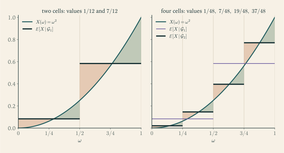
Two things visible in Figure 6.1 will become theorems. First, averaging the finer step function over the coarser cells returns the coarser step function: \(\tfrac12(\tfrac1{48}+\tfrac7{48})=\tfrac1{12}\) and \(\tfrac12(\tfrac{19}{48}+\tfrac{37}{48})=\tfrac7{12}\) . That is the tower property. Second, the step functions approach \(X\) as the partition is refined. The mean square error is

\[ \mathbb E\bigl(X-\mathbb E[X\mid\mathcal G_1]\bigr)^2=\frac{19}{720}\approx 0.0264,\qquad \mathbb E\bigl(X-\mathbb E[X\mid\mathcal G_2]\bigr)^2=\frac{79}{11520}\approx 0.0069, \]

roughly a factor of four smaller at each refinement. Chapter 7 proves that such approximations converge for every integrable \(X\) .

6.2 The definition, and why it can be met

The two properties that characterized the conditional expectation in the finite case make sense for any sub-sigma-algebra, and they are taken as the definition.

Condition (a) says that \(Y\) uses only the information in \(\mathcal G\) ; condition (b) says that it is correct on average over every event that this information can describe. By the Doob–Dynkin theorem (Theorem 1.5), \(\mathbb E[X\mid Z]=g(Z)\) for some measurable function \(g\) , and \(g(z)\) is what a first course writes as \(\mathbb E[X\mid Z=z]\) . The function \(g\) is determined only up to sets of \(\mathbb P_Z\) -measure zero, so its value at an individual point has no meaning when that point is not an atom of the law of \(Z\) .

Existence rests on the Radon–Nikodym theorem of Measure Theory: if \(\nu\) and \(\mu\) are finite measures on one measurable space and \(\nu(G)=0\) whenever \(\mu(G)=0\) , then there is a nonnegative measurable function \(Y\) with \(\nu(G)=\int_GY\,d\mu\) for every measurable \(G\) (math.measure-theory.radon-nikodym-theorem).

The step that matters is the choice of the measurable space. On \((\Omega,\mathcal F)\) the measure \(G\mapsto\mathbb E[X;G]\) has the density \(X\) , trivially. Applying the theorem on the smaller space \((\Omega,\mathcal G)\) forces the density to be \(\mathcal G\) -measurable, and a \(\mathcal G\) -measurable density for the same measure, restricted to \(\mathcal G\) , is precisely the conditional expectation. Conditioning is the coarsening of a density.

Because of uniqueness, every statement about \(\mathbb E[X\mid\mathcal G]\) is to be read as holding almost surely, for any version. The defining identity (b) extends from indicators to bounded test variables by the standard ladder of Chapter 1.

6.3 The rules of calculation

Almost nothing about conditional expectation is ever proved by computing a density. One proposes a candidate and checks conditions (a) and (b); uniqueness does the rest. All of the following rules are proved in that way.

The tower property is the rule of iterated expectations of a first course (math.probability-theory.tower-property), now free of densities: coarsening in two steps is the same as coarsening in one. Its order matters. The smaller sigma-algebra always wins, and when neither sigma-algebra contains the other the two iterated conditional expectations generally differ (Exercise 5).

The convergence theorems carry over, with almost sure convergence of the conditional expectations in the conclusion.

The supremum had to be countable because each inequality holds only almost surely, and an uncountable union of null events need not be null. With \(\varphi(x)=\lvert x\rvert^p\) for \(p\ge 1\) , the inequality reads \(\lvert\mathbb E[X\mid\mathcal G]\rvert^p\le\mathbb E[\lvert X\rvert^p\mid\mathcal G]\) , and taking expectations,

Conditioning never increases an \(L^p\) norm.

When the information is a random variable and a joint density is available, the definition returns the formula of a first course, and the proof is the verification of (b) on a generating \(\pi\) -system.

6.4 The best predictor

For square-integrable variables conditional expectation has a geometric meaning that explains why it is the right notion of an estimate based on partial information.

In the language of Functional Analysis, the \(\mathcal G\) -measurable members of \(L^2\) form a closed subspace, and \(\mathbb E[\,\cdot\mid\mathcal G]\) is the orthogonal projection onto it. One can run the logic in reverse: the projection theorem for Hilbert spaces (math.functional-analysis.hilbert-projection-theorem), which needs only that the subspace be closed, produces \(\mathbb E[X\mid\mathcal G]\) for \(X\in L^2\) without the Radon–Nikodym theorem, and monotone limits then extend it to \(L^1\) . Either route leads to the same object.

Taking \(Z=\mathbb E X\) in the theorem gives the decomposition of variance into the part explained by \(\mathcal G\) and the part left over:

6.5 A uniformly integrable family

The last result of the chapter connects conditioning with Chapter 5 and will be used in the proof of the martingale convergence theorems.

The whole conditional law of \(X\) given \(\mathcal G\) , not only its mean, can be defined along the same lines: for real-valued \(X\) there is a family of probability measures \(\mu_\omega\) on \(\mathbb R\) , depending measurably on \(\omega\) through \(\mathcal G\) , such that \(\omega\mapsto\int h\,d\mu_\omega\) is a version of \(\mathbb E[h(X)\mid\mathcal G]\) for every bounded measurable \(h\) . Such regular conditional distributions exist for variables with values in well-behaved spaces. We state this without proof and do not use it; every argument in this book works with conditional expectations directly.

With conditional expectation in hand, information can be allowed to grow with time. If \(\mathcal F_1\subseteq\mathcal F_2\subseteq\cdots\) and \(X\) is integrable, the estimates \(\mathbb E[X\mid\mathcal F_n]\) form a sequence in which, by the tower property, each term is the conditional expectation of the next given the earlier information. What can be said about every sequence with that property?

Exercises

1. On \(\Omega=\{1,\dots,6\}\) with the uniform probability let \(X(\omega)=\omega^2\) and let \(\mathcal G\) be generated by the partition \(\{1,2\}\) , \(\{3,4,5,6\}\) . Compute \(\mathbb E[X\mid\mathcal G]\) and verify directly that its mean is \(\mathbb E X\) .

   Answer

   \(\mathbb E[X\mid\mathcal G]\) equals \((1+4)/2=5/2\) on \(\{1,2\}\) and \((9+16+25+36)/4=43/2\) on \(\{3,4,5,6\}\) . Its mean is \(\tfrac26\cdot\tfrac52+\tfrac46\cdot\tfrac{43}{2}=\tfrac{91}{6}=\mathbb E X\) .

2. Show from the definition that \(\mathbb E[X\mid\mathcal G]=\mathbb E X\) when \(\mathcal G=\{\emptyset,\Omega\}\) and \(\mathbb E[X\mid\mathcal G]=X\) when \(\mathcal G=\mathcal F\) , and say which property of Theorem 6.4 each is a special case of.

   Answer

   For the trivial sigma-algebra the only measurable functions are constants, and condition (b) with \(G=\Omega\) forces the constant \(\mathbb E X\) ; this is Theorem 6.4(g), since every variable is independent of the trivial sigma-algebra. For \(\mathcal G=\mathcal F\) the variable \(X\) itself satisfies (a) and (b); this is Theorem 6.4(d).

3. Let \(Y\) and \(Y'\) be integrable and \(\mathcal G\) -measurable with \(\mathbb E[Y;G]\le\mathbb E[Y';G]\) for every \(G\in\mathcal G\) . Prove that \(Y\le Y'\) almost surely, and deduce the uniqueness part of Theorem 6.2.

   Solution

   Let \(G=\{Y>Y'\}\) . Both variables are \(\mathcal G\) -measurable, so \(G\in\mathcal G\) , and the hypothesis gives \(\mathbb E[Y-Y';G]\le 0\) . But \((Y-Y')\mathbf 1_G\ge 0\) everywhere, so its expectation is also at least \(0\) ; hence \(\mathbb E[(Y-Y')\mathbf 1_G]=0\) . A nonnegative random variable with zero expectation vanishes almost surely, and \((Y-Y')\mathbf 1_G\) is strictly positive on \(G\) , so \(\mathbb P(G)=0\) . That is, \(Y\le Y'\) almost surely.

   For uniqueness, let \(Y\) and \(Y'\) both be versions of \(\mathbb E[X\mid\mathcal G]\) . Then \(\mathbb E[Y;G]=\mathbb E[X;G]=\mathbb E[Y';G]\) for all \(G\in\mathcal G\) , so the hypothesis holds in both directions, and the first part gives \(Y\le Y'\) and \(Y'\le Y\) almost surely. The same comparison proves monotonicity of conditional expectation: it is the tool behind every “almost surely” inequality between \(\mathcal G\) -measurable variables.

4. Prove the conditional Chebyshev inequality: for \(X\in L^2\) and \(a>0\) , \(\mathbb P(\lvert X\rvert\ge a\mid\mathcal G)\le a^{-2}\,\mathbb E[X^2\mid\mathcal G]\) almost surely.

   Hint

   Pointwise \(a^2\mathbf 1_{\{\lvert X\rvert\ge a\}}\le X^2\) . Apply monotonicity and linearity of \(\mathbb E[\,\cdot\mid\mathcal G]\) .

5. On \(\Omega=\{1,2,3\}\) with the uniform probability let \(\mathcal G=\sigma(\{1,2\})\) , \(\mathcal H=\sigma(\{2,3\})\) , and \(X=\mathbf 1_{\{1\}}\) . Compute \(\mathbb E[\mathbb E[X\mid\mathcal G]\mid\mathcal H]\) and \(\mathbb E[\mathbb E[X\mid\mathcal H]\mid\mathcal G]\) and explain why this does not contradict the tower property.

   Solution

   The cells of \(\mathcal G\) are \(\{1,2\}\) and \(\{3\}\) ; the cells of \(\mathcal H\) are \(\{1\}\) and \(\{2,3\}\) . Write a random variable as the triple of its values at \(1,2,3\) , so \(X=(1,0,0)\) .

   Averaging over the cells of \(\mathcal G\) : \(\mathbb E[X\mid\mathcal G]=(\tfrac12,\tfrac12,0)\) . Averaging that over the cells of \(\mathcal H\) : the value at \(1\) is kept, and on \(\{2,3\}\) the average of \(\tfrac12\) and \(0\) is \(\tfrac14\) , so

   \[ \mathbb E\bigl[\mathbb E[X\mid\mathcal G]\mid\mathcal H\bigr]=(\tfrac12,\tfrac14,\tfrac14). \]

   In the other order: \(X\) is already constant on the cells of \(\mathcal H\) , so \(\mathbb E[X\mid\mathcal H]=(1,0,0)\) , and averaging over the cells of \(\mathcal G\) gives

   \[ \mathbb E\bigl[\mathbb E[X\mid\mathcal H]\mid\mathcal G\bigr]=(\tfrac12,\tfrac12,0). \]

   The two results differ. This does not contradict Theorem 6.4(e), whose hypothesis is that one sigma-algebra contains the other; here neither does, since \(\{1,2\}\notin\mathcal H\) and \(\{2,3\}\notin\mathcal G\) . Both iterated expectations have mean \(\tfrac13=\mathbb E X\) , as they must, but conditional expectations given unrelated sigma-algebras do not commute.

6. Let \((X,Y)\) have joint density \(f(x,y)=x+y\) on the unit square. Find \(\mathbb E[X\mid Y]\) and verify that its expectation is \(\mathbb E X\) .

   Solution

   The marginal density of \(Y\) is \(f_Y(y)=\int_0^1(x+y)\,dx=\tfrac12+y\) , and \(\int_0^1x(x+y)\,dx=\tfrac13+\tfrac y2\) . By the density formula stated after Example 6.3,

   \[ \mathbb E[X\mid Y]=g(Y),\qquad g(y)=\frac{\tfrac13+\tfrac y2}{\tfrac12+y}=\frac{2+3y}{3+6y}. \]

   To verify the mean, integrate \(g\) against the law of \(Y\) : the denominator cancels the density, and

   \[ \mathbb E\,g(Y)=\int_0^1\Bigl(\frac13+\frac y2\Bigr)dy=\frac13+\frac14=\frac7{12}, \]

   which equals \(\mathbb E X=\int_0^1x(x+\tfrac12)\,dx=\tfrac13+\tfrac14\) . The conditional expectation decreases from \(g(0)=\tfrac23\) to \(g(1)=\tfrac59\) : a large value of \(Y\) makes a large value of \(X\) slightly less likely under this density, which is consistent with the negative covariance \(\mathbb E[XY]-\mathbb E X\,\mathbb E Y=\tfrac13-\tfrac{49}{144}=-\tfrac1{144}\) .

7. Let \(X_1,\dots,X_n\) be i.i.d. and integrable with sum \(S\) . Prove that \(\mathbb E[X_1\mid S]=S/n\) using only the defining property and the symmetry of the joint law.

   Solution

   By Theorem 1.5 there is a measurable \(g\) with \(\mathbb E[X_1\mid S]=g(S)\) . Fix \(i\) and a bounded measurable \(h\) . The vector obtained from \((X_1,\dots,X_n)\) by exchanging the first and \(i\) -th coordinates has the same joint law, because the joint law is a product of identical factors, and \(S\) is unchanged by the exchange. Therefore

   \[ \mathbb E[X_i\,h(S)]=\mathbb E[X_1\,h(S)]=\mathbb E[g(S)\,h(S)], \]

   the second equality by Proposition 6.3. Taking \(h=\mathbf 1_B\) shows that \(g(S)\) satisfies the defining property for \(X_i\) on every event \(\{S\in B\}\) of \(\sigma(S)\) . So \(\mathbb E[X_i\mid S]=g(S)\) for every \(i\) , with the same \(g\) . Summing over \(i\) and using linearity and Theorem 6.4(d),

   \[ n\,g(S)=\sum_{i=1}^n\mathbb E[X_i\mid S]=\mathbb E[S\mid S]=S . \]

   Hence \(\mathbb E[X_1\mid S]=S/n\) . Independence was used only to obtain a joint law invariant under permutations; no density and no computation of the law of \(S\) was needed.

8. Let \(X\) and \(Y\) be independent exponential variables with rate \(1\) and \(m=X\wedge Y\) . Find \(\mathbb E[X\mid m]\) by proposing a candidate and verifying the averaging identity on the events \(\{m>t\}\) .

   Answer

   \(\mathbb E[X\mid m]=m+\tfrac12\) : given the minimum, \(X\) is the minimum with probability \(\tfrac12\) , and otherwise exceeds it by an independent exponential amount. Check: \(\mathbb E[X;m>t]=\mathbb E[X;X>t]\,\mathbb P(Y>t)=(t+1)e^{-2t}\) , and since \(m\) is exponential with rate \(2\) , \(\mathbb E[m+\tfrac12;m>t]=(t+\tfrac12)e^{-2t}+\tfrac12e^{-2t}=(t+1)e^{-2t}\) .

9. Show by example that \(\mathbb E[X\mid\mathcal G]=\mathbb E X\) does not imply that \(X\) is independent of \(\mathcal G\) , using a variable from Chapter 2.

   Answer

   Take \(X\) uniform on \(\{-1,0,1\}\) and \(\mathcal G=\sigma(X^2)\) , as in Example 2.3. On \(\{X^2=1\}\) the average of \(X\) is \(0\) , and on \(\{X^2=0\}\) it is \(0\) , so \(\mathbb E[X\mid\mathcal G]=0=\mathbb E X\) ; but \(X\) is not independent of \(X^2\) .

10. Prove the conditional Cauchy–Schwarz inequality \(\bigl(\mathbb E[\lvert XY\rvert\mid\mathcal G]\bigr)^2\le\mathbb E[X^2\mid\mathcal G]\,\mathbb E[Y^2\mid\mathcal G]\) for \(X,Y\in L^2\) .

    Hint

    For rational \(\lambda\) , \(0\le\mathbb E[(\lvert X\rvert+\lambda\lvert Y\rvert)^2\mid\mathcal G]\) is a quadratic in \(\lambda\) with \(\mathcal G\) -measurable coefficients, valid for all rational \(\lambda\) outside one null event; its discriminant is nonpositive there.

11. For the pair of Example 6.3 a student writes “\(\mathbb E[X\mid Y]=\mathbb E X=2/3\) , since \(\mathbb E[\mathbb E[X\mid Y]]=\mathbb E X\) .” Show that the constant \(2/3\) violates the defining property on a specific event, state what the quoted identity actually says, and compute the variance of the correct conditional expectation.

    Solution

    If the constant \(\tfrac23\) were a version of \(\mathbb E[X\mid Y]\) , the defining property would give \(\mathbb E[X;Y\le t]=\tfrac23\,\mathbb P(Y\le t)\) for every \(t\) . By Example 6.3, \(\mathbb E[X;Y\le t]=t-t^3/3\) , and \(\mathbb P(Y\le t)=\int_0^t2(1-y)\,dy=2t-t^2\) . At \(t=\tfrac12\) the left side is \(\tfrac12-\tfrac1{24}=\tfrac{11}{24}\) and the right side is \(\tfrac23\cdot\tfrac34=\tfrac12\) . They differ, so the constant fails condition (b) on the event \(\{Y\le\tfrac12\}\) .

    The identity \(\mathbb E[\mathbb E[X\mid Y]]=\mathbb E X\) says that the random variable \(\mathbb E[X\mid Y]\) has mean \(\mathbb E X=\tfrac23\) . It does not say that the random variable is constant; that would hold if \(X\) were independent of \(Y\) , which is not the case here. The correct conditional expectation is \(\tfrac12(1+Y)\) , whose mean is indeed \(\tfrac12(1+\tfrac13)=\tfrac23\) , and whose variance is

    \[ \operatorname{Var}\bigl(\tfrac12(1+Y)\bigr)=\tfrac14\operatorname{Var}(Y)=\tfrac14\Bigl(\tfrac16-\tfrac19\Bigr)=\tfrac1{72}, \]

    using \(\mathbb E Y=\tfrac13\) and \(\mathbb E Y^2=\int_0^1y^2\cdot 2(1-y)\,dy=\tfrac16\) . A positive variance is the quantitative sign that the conditional expectation is a genuine random variable.

12. Let \(\mathcal H\subseteq\mathcal G\) and \(X\in L^2\) . Prove that \(\mathbb E(X-\mathbb E[X\mid\mathcal G])^2\le\mathbb E(X-\mathbb E[X\mid\mathcal H])^2\) , with the difference equal to \(\mathbb E(\mathbb E[X\mid\mathcal G]-\mathbb E[X\mid\mathcal H])^2\) .

    Solution

    Put \(Y_{\mathcal G}=\mathbb E[X\mid\mathcal G]\) and \(Y_{\mathcal H}=\mathbb E[X\mid\mathcal H]\) . Both are in \(L^2\) by the conditional Jensen inequality. Since \(\mathcal H\subseteq\mathcal G\) , the variable \(Y_{\mathcal H}\) is \(\mathcal G\) -measurable, so it is an admissible competitor \(Z\) in Theorem 6.8 applied with the sigma-algebra \(\mathcal G\) :

    \[ \mathbb E(X-Y_{\mathcal H})^2=\mathbb E(X-Y_{\mathcal G})^2+\mathbb E(Y_{\mathcal G}-Y_{\mathcal H})^2 . \]

    The last term is nonnegative, which gives the inequality and identifies the difference. In words: more information never worsens the best mean-square prediction, and the improvement is exactly the mean square of the revision \(Y_{\mathcal G}-Y_{\mathcal H}\) . By the tower property \(Y_{\mathcal H}=\mathbb E[Y_{\mathcal G}\mid\mathcal H]\) , so the identity is also the variance decomposition for \(Y_{\mathcal G}\) given \(\mathcal H\) .

13. Let \(N\) be a random variable with values in \(\{1,2,\dots\}\) and finite variance, independent of the i.i.d. square-integrable sequence \(X_1,X_2,\dots\) with mean \(\mu\) and variance \(\sigma^2\) , and let \(S=X_1+\dots+X_N\) . Prove that \(\mathbb E[S\mid N]=N\mu\) and \(\operatorname{Var}(S)=\sigma^2\,\mathbb E N+\mu^2\operatorname{Var}(N)\) , and evaluate the variance when \(N\) is uniform on \(\{1,2,3\}\) and the \(X_i\) are fair coin indicators.

    Solution

    Let \(\mathcal G=\sigma(N)\) . The sequence \(\mathbf X=(X_1,X_2,\dots)\) is a random element of \(\mathbb R^{\mathbb N}\) independent of \(\mathcal G\) , and \(S=h(N,\mathbf X)\) with \(h(n,\mathbf x)=x_1+\dots+x_n\) . Apply Proposition 6.7 to \(h\) and to \(h^2\) ; integrability follows from the nonnegative case applied to \(\lvert h\rvert\) and \(h^2\) , because the frozen expectations are

    \[ H_1(n)=\mathbb E[X_1+\dots+X_n]=n\mu,\qquad H_2(n)=\mathbb E(X_1+\dots+X_n)^2=n\sigma^2+n^2\mu^2, \]

    and \(N\) has a finite second moment. Hence \(\mathbb E[S\mid N]=N\mu\) and \(\mathbb E[S^2\mid N]=N\sigma^2+N^2\mu^2\) . Taking expectations,

    \[ \operatorname{Var}(S)=\sigma^2\,\mathbb E N+\mu^2\,\mathbb E N^2-\mu^2(\mathbb E N)^2=\sigma^2\,\mathbb E N+\mu^2\operatorname{Var}(N). \]

    The two terms are the two parts of the variance decomposition of Section 6.4: the average conditional variance \(\mathbb E[N\sigma^2]\) and the variance \(\mu^2\operatorname{Var}(N)\) of the conditional mean. For \(N\) uniform on \(\{1,2,3\}\) and fair coin indicators, \(\mu=\tfrac12\) , \(\sigma^2=\tfrac14\) , \(\mathbb E N=2\) , \(\operatorname{Var}(N)=\tfrac23\) , so \(\operatorname{Var}(S)=\tfrac12+\tfrac16=\tfrac23\) .

14. State and prove a conditional form of Fatou’s lemma, deducing it from Theorem 6.5(a).

    Hint

    Statement: if \(X_n\ge 0\) are integrable and \(\liminf_nX_n\) is integrable, then \(\mathbb E[\liminf_nX_n\mid\mathcal G]\le\liminf_n\mathbb E[X_n\mid\mathcal G]\) almost surely. Apply Theorem 6.5(a) to \(\inf_{k\ge n}X_k\uparrow\liminf_nX_n\) and use monotonicity.

15. Let \(X\ge 0\) be integrable. Prove that \(\{X>0\}\subseteq\{\mathbb E[X\mid\mathcal G]>0\}\) up to a null event, and that \(\mathbb E[X\mid\mathcal G]=0\) almost surely implies \(X=0\) almost surely.

    Hint

    Let \(G=\{\mathbb E[X\mid\mathcal G]=0\}\in\mathcal G\) . Then \(\mathbb E[X;G]=\mathbb E[\mathbb E[X\mid\mathcal G];G]=0\) , so \(X=0\) almost surely on \(G\) .

16. Let \(X\) be integrable and let \(\mathcal G_1,\mathcal G_2,\dots\) be sub-sigma-algebras such that \(\mathbb E[X\mid\mathcal G_n]\) converges in probability to some \(Y\) . Prove that the convergence also holds in \(L^1\) .

    Answer

    By Theorem 6.9 the sequence \(\mathbb E[X\mid\mathcal G_n]\) is uniformly integrable, and it converges in probability, so Theorem 5.6 gives convergence in \(L^1\) .

17. Let \(X,Y\in L^2\) satisfy \(\mathbb E[X\mid Y]=Y\) and \(\mathbb E[Y\mid X]=X\) . Prove that \(X=Y\) almost surely.

    Solution

    All the products below are integrable by the Cauchy–Schwarz inequality. Since \(Y\) is \(\sigma(Y)\) -measurable, taking out what is known and then expectations gives

    \[ \mathbb E[XY]=\mathbb E\bigl[\mathbb E[XY\mid Y]\bigr]=\mathbb E\bigl[Y\,\mathbb E[X\mid Y]\bigr]=\mathbb E[Y^2]. \]

    By the symmetric argument with the roles exchanged, \(\mathbb E[XY]=\mathbb E\bigl[X\,\mathbb E[Y\mid X]\bigr]=\mathbb E[X^2]\) . Therefore

    \[ \mathbb E(X-Y)^2=\mathbb E X^2-2\,\mathbb E[XY]+\mathbb E Y^2=\mathbb E[XY]-2\,\mathbb E[XY]+\mathbb E[XY]=0, \]

    and a nonnegative variable with zero expectation vanishes almost surely, so \(X=Y\) almost surely. Geometrically: \(Y\) is the projection of \(X\) onto the functions of \(Y\) and \(X\) is the projection of \(Y\) onto the functions of \(X\) ; projections shorten, so \(\lVert Y\rVert_2\le\lVert X\rVert_2\le\lVert Y\rVert_2\) , and a projection that does not shorten moves nothing.

18. On the unit square with Lebesgue measure let \(\mathcal G\) be the sigma-algebra of sets \(B\times[0,1)\) with \(B\) Borel, and let \(X\) be integrable. Prove that \(\mathbb E[X\mid\mathcal G](\omega_1,\omega_2)=\int_0^1X(\omega_1,t)\,dt\) .

    Solution

    By Fubini’s theorem, for almost every \(\omega_1\) the function \(t\mapsto X(\omega_1,t)\) is integrable, and \(Y(\omega_1,\omega_2)=\int_0^1X(\omega_1,t)\,dt\) , set equal to \(0\) for the exceptional \(\omega_1\) , is a measurable function of \(\omega_1\) alone. A function of \(\omega_1\) alone is \(\mathcal G\) -measurable, since its level sets have the form \(B\times[0,1)\) . It is integrable, because \(\int\lvert Y\rvert\le\iint\lvert X\rvert\) . For \(G=B\times[0,1)\) , Fubini’s theorem gives

    \[ \mathbb E[Y;G]=\int_B\Bigl(\int_0^1Y(\omega_1,\omega_2)\,d\omega_2\Bigr)d\omega_1=\int_B\Bigl(\int_0^1X(\omega_1,t)\,dt\Bigr)d\omega_1=\mathbb E[X;G], \]

    where the inner integral of \(Y\) over \(\omega_2\) is just \(Y\) , which does not depend on \(\omega_2\) . Both conditions of Definition 6.1 hold, so \(Y\) is a version of \(\mathbb E[X\mid\mathcal G]\) . This is conditional expectation in its most literal form: integrate out the coordinate that is not observed. It is also the case \(S=T=[0,1)\) of Proposition 6.7.