Push a child on a swing once per swing and a gentle hand soon produces a large arc. Push with the same force at a slightly different rhythm and the swing alternately gains and loses, never getting far. Push much faster than the swing’s own rhythm and almost nothing happens. The force is the same in the three cases. Only its timing differs.
A swing through small angles, a mass on a spring, a tuned circuit, and a building in an earthquake are all described by \(my''+cy'+ky=F(t)\) , a linear equation with constant coefficients driven by an external forcing term. This chapter asks how the response \(y\) depends on the forcing \(F\) . The answer has two layers. The algebraic layer is a set of methods for finding one solution of the forced equation, since by linearity one is enough. The physical layer is what those solutions say when \(F\) oscillates: the response is governed by a single complex number, \(1/P(i\omega)\) , whose size and angle are the amplification and the delay at forcing frequency \(\omega\) , and whose behaviour near the system’s natural frequency is resonance.
5.1 One particular solution is enough
Keep the notation \(L[y]=y''+p(t)y'+q(t)y\) of Chapter 4, with \(p\) , \(q\) , \(g\) continuous on an interval \(I\) .
Theorem 5.1 (structure of the forced equation). Let \(y_p\) be any one solution of \(L[y]=g\) on \(I\) , and let \(\{y_1,y_2\}\) be a fundamental set for \(L[y]=0\) . Then the solutions of \(L[y]=g\) on \(I\) are exactly the functions
Moreover, if \(L[y_a]=g_a\) and \(L[y_b]=g_b\) , then \(L[y_a+y_b]=g_a+g_b\) .
Proof. By linearity (Theorem 4.2), \(L[y_p+c_1y_1+c_2y_2]=g+0+0=g\) . Conversely, if \(L[y]=g\) then \(L[y-y_p]=g-g=0\) , so \(y-y_p\) is a solution of the homogeneous equation and, by Theorem 4.5, equals \(c_1y_1+c_2y_2\) for some constants. The last statement is linearity once more.
The function \(y_p\) is called a particular solution and \(y_h=c_1y_1+c_2y_2\) the complementary solution. The second statement, superposition of forcings, lets a complicated \(g\) be split into simple pieces treated one at a time. So the whole problem is reduced to producing one solution for each simple kind of forcing, and for constant coefficients the simplest kind is an exponential.
5.2 Exponential forcing and undetermined coefficients
Let \(L[y]=ay''+by'+cy\) with real constants, \(a\ne0\) , and characteristic polynomial \(P(r)=ar^2+br+c\) . Section 4.3 showed that \(L[e^{st}]=P(s)e^{st}\) for every real or complex number \(s\) . If \(P(s)\ne0\) , dividing by \(P(s)\) solves \(L[y]=e^{st}\) at a stroke. If \(P(s)=0\) the exponential is itself a solution of the homogeneous equation and cannot produce a nonzero right-hand side; something else is needed.
Theorem 5.2 (exponential response). Let \(s\) be a real or complex number.
(a) If \(P(s)\ne0\) , then \(y_p=\dfrac{e^{st}}{P(s)}\) satisfies \(L[y_p]=e^{st}\) .
(b) If \(P(s)=0\) and \(P'(s)\ne0\) , then \(y_p=\dfrac{t\,e^{st}}{P'(s)}\) satisfies \(L[y_p]=e^{st}\) .
(c) If \(P(s)=P'(s)=0\) , then \(y_p=\dfrac{t^2e^{st}}{2a}\) satisfies \(L[y_p]=e^{st}\) .
Proof. Part (a) is the identity \(L[e^{st}]=P(s)e^{st}\) . For the others compute directly. With \(y=te^{st}\) : \(y'=(1+st)e^{st}\) , \(y''=(2s+s^2t)e^{st}\) , so
With \(y=t^2e^{st}\) : \(y'=(2t+st^2)e^{st}\) , \(y''=(2+4st+s^2t^2)e^{st}\) , so
Setting \(P(s)=0\) in the first identity gives (b), and \(P(s)=P'(s)=0\) in the second gives (c).
Case (a) says that a system driven by an exponential it does not itself produce responds with the same exponential, scaled by \(1/P(s)\) . Cases (b) and (c) say that when the forcing matches one of the system’s own modes, the response acquires a factor of \(t\) , or \(t^2\) for a double root. That extra factor is the mathematical form of resonance.
Sinusoidal forcing is included, through complex exponentials. Since \(\cos\omega t\) is the real part of \(e^{i\omega t}\) and the coefficients of \(L\) are real, the real part of a solution of \(L[z]=e^{i\omega t}\) is a solution of \(L[y]=\cos\omega t\) , and its imaginary part solves \(L[y]=\sin\omega t\) . One complex division replaces a pair of simultaneous equations for the coefficients of a cosine and a sine.
Example 5.1: Forcing off and on a characteristic root
For \(y''-y=e^{2t}\) we have \(P(r)=r^2-1\) and \(P(2)=3\ne0\) , so \(y_p=\tfrac13e^{2t}\) , and the general solution is \(y=\tfrac13e^{2t}+c_1e^{t}+c_2e^{-t}\) .
For \(y''-y=e^{t}\) the forcing exponent \(s=1\) is a root: \(P(1)=0\) , while \(P'(r)=2r\) gives \(P'(1)=2\) . Part (b) gives \(y_p=\tfrac12te^{t}\) . Check: \(y_p'=\tfrac12(1+t)e^{t}\) , \(y_p''=\tfrac12(2+t)e^{t}\) , and \(y_p''-y_p=e^{t}\) . A trial of the form \(Ae^{t}\) would have failed, since \(L[Ae^{t}]=0\) for every \(A\) .
Example 5.2: A sinusoidal input by complex replacement
Find a particular solution of \(y''+2y'+5y=4\cos2t\) and describe it.
Replace the right side by \(4e^{2it}\) . Here \(P(r)=r^2+2r+5\) and
so a complex solution is \(z_p=\dfrac{4e^{2it}}{1+4i}\) . Multiply numerator and denominator by \(1-4i\) :
For the amplitude and delay, write \(1+4i=\sqrt{17}\,e^{i\phi}\) with \(\phi=\arctan4\approx1.326\) . Then \(z_p=\dfrac{4}{\sqrt{17}}e^{i(2t-\phi)}\) and
The response has the frequency of the input, amplitude \(0.970\) against the input’s \(4\) , and it lags by \(1.326\) radians, about \(76\) degrees. The general solution adds \(e^{-t}(c_1\cos2t+c_2\sin2t)\) , which decays; after a few time units every solution is indistinguishable from \(y_p\) .
The same idea extends to forcing terms that are products of polynomials, exponentials, and sines or cosines. All derivatives of such a function are combinations of finitely many functions of the same kind, so one may guess a combination of those functions with unknown coefficients, substitute, and solve for the coefficients. This is the method of undetermined coefficients.
| Forcing \(g(t)\) | Trial particular solution |
|---|---|
| polynomial of degree \(n\) | \(t^{k}\,(A_nt^n+\dots+A_1t+A_0)\) |
| polynomial of degree \(n\) times \(e^{st}\) | \(t^{k}\,(A_nt^n+\dots+A_0)\,e^{st}\) |
| \(e^{\lambda t}\cos\mu t\) or \(e^{\lambda t}\sin\mu t\) | \(t^{k}\,e^{\lambda t}(A\cos\mu t+B\sin\mu t)\) |
In each row \(k\) is the multiplicity of the forcing exponent as a root of the characteristic polynomial: the exponent is \(0\) in the first row, \(s\) in the second, and \(\lambda+i\mu\) in the third; \(k=0\) if it is not a root, \(1\) for a simple root, \(2\) for a double root. The factor \(t^{k}\) is the general form of the extra factors in Theorem 5.2.
Example 5.3: A doubly resonant forcing
Solve \(y''-2y'+y=te^{t}\) .
The characteristic polynomial is \((r-1)^2\) , so \(s=1\) is a double root and the complementary solution is \((c_1+c_2t)e^{t}\) . The table prescribes the trial \(t^2(At+B)e^{t}\) . The coefficients are found fastest by writing \(y=e^{t}v\) . Then \(y'=e^{t}(v'+v)\) , \(y''=e^{t}(v''+2v'+v)\) , and
The equation becomes \(v''=t\) , with particular solution \(v=t^3/6\) . Hence
In the trial’s notation \(A=1/6\) and \(B=0\) . The two constants of integration of \(v''=t\) reproduce the complementary solution.
Common mistake. Using a trial that already solves the homogeneous equation. For \(y''+4y=\sin2t\) the natural guess \(A\cos2t+B\sin2t\) gives \(L[y]=0\) identically, and the “equation” for the coefficients reads \(0=\sin2t\) . This is not a sign that no solution exists. The forcing exponent \(2i\) is a characteristic root, so \(k=1\) and the trial must be \(t\,(A\cos2t+B\sin2t)\) . Before choosing a trial, write down the characteristic roots and compare them with the exponent of the forcing.
5.3 Variation of parameters
Undetermined coefficients requires constant coefficients and a forcing term of the special kinds in the table. For \(y''+y=\sec t\) , or for an equation with variable coefficients, it has nothing to offer. The following method works whenever a fundamental set is known.
Theorem 5.3 (variation of parameters). Let \(\{y_1,y_2\}\) be a fundamental set for \(y''+p(t)y'+q(t)y=0\) on \(I\) , with Wronskian \(W\) , and let \(g\) be continuous on \(I\) . Then
is a solution of \(y''+p(t)y'+q(t)y=g(t)\) on \(I\) .
Proof. Look for a solution \(y=u_1y_1+u_2y_2\) in which the constants of the complementary solution are replaced by functions. There are two unknown functions and one equation, so one further condition may be imposed, and it is chosen to keep second derivatives of \(u_1,u_2\) out of the calculation: require
Then \(y'=u_1y_1'+u_2y_2'\) and \(y''=u_1y_1''+u_2y_2''+u_1'y_1'+u_2'y_2'\) . Substituting and using \(L[y_1]=L[y_2]=0\) ,
So \(L[y]=g\) holds if \(u_1'\) , \(u_2'\) satisfy the linear system
Its determinant is \(W\ne0\) , and Cramer’s rule gives \(u_1'=-y_2g/W\) and \(u_2'=y_1g/W\) . These are continuous on \(I\) , so they have antiderivatives, and the resulting \(y\) is the stated \(y_p\) .
The equation must be in normal form, with leading coefficient \(1\) , before \(g\) is read off. Different choices of the constants of integration change \(y_p\) by a solution of the homogeneous equation, which is harmless. If the integrals are taken from \(t_0\) to \(t\) , the formula can be written with a single integral,
and this particular solution has \(y_p(t_0)=0\) and \(y_p'(t_0)=0\) . The response at time \(t\) is a weighted sum of the forcing at all earlier times \(s\) . For constant coefficients the weight depends only on the elapsed time \(t-s\) , a fact that Chapter 6 turns into the convolution theorem.
Example 5.4: A forcing outside the table
Solve \(y''+y=\sec t\) on \((-\pi/2,\pi/2)\) .
A fundamental set is \(y_1=\cos t\) , \(y_2=\sin t\) , with \(W=1\) , and \(g=\sec t\) is continuous on the interval. Then
so \(u_1=\ln(\cos t)\) , valid because \(\cos t>0\) on the interval, and \(u_2=t\) . Therefore
Check: \(y_p'=-\sin t\ln(\cos t)+t\cos t\) , since the two terms \(\mp\sin t\) cancel, and \(y_p''=-\cos t\ln(\cos t)+\sin t\tan t+\cos t-t\sin t\) . Adding \(y_p\) leaves \(\sin t\tan t+\cos t=\dfrac{\sin^2t+\cos^2t}{\cos t}=\sec t\) .
The solution is confined to an interval between consecutive singularities of the forcing, as Theorem 4.1 requires. When both methods apply, undetermined coefficients is usually quicker; variation of parameters is the general tool and the one that explains the structure.
5.4 Undamped forcing: beats and pure resonance
Now the oscillator. Without damping, and with forcing amplitude \(F\) per unit mass, the model is
a system at rest switched on at time zero. The characteristic roots are \(\pm i\omega_0\) .
Forcing off resonance, \(\omega\ne\omega_0\) . Theorem 5.2(a) with \(s=i\omega\) and \(P(i\omega)=\omega_0^2-\omega^2\) gives \(y_p=\dfrac{F\cos\omega t}{\omega_0^2-\omega^2}\) . Adding \(c_1\cos\omega_0t+c_2\sin\omega_0t\) and fitting the rest data gives \(c_2=0\) and \(c_1=-F/(\omega_0^2-\omega^2)\) :
The second form uses \(\cos\alpha-\cos\beta=2\sin\frac{\beta-\alpha}{2}\sin\frac{\beta+\alpha}{2}\) . When \(\omega\) is close to \(\omega_0\) it shows a fast oscillation at the mean frequency \(\tfrac12(\omega_0+\omega)\) whose amplitude is modulated slowly, at the frequency \(\tfrac12\lvert\omega_0-\omega\rvert\) . The swelling and fading are called beats. The envelope returns to zero every \(2\pi/\lvert\omega_0-\omega\rvert\) units of time, and its maximum, \(2F/\lvert\omega_0^2-\omega^2\rvert\) , grows without bound as \(\omega\to\omega_0\) .
Forcing at resonance, \(\omega=\omega_0\) . Now \(i\omega_0\) is a simple root, \(P'(i\omega_0)=2i\omega_0\) , and Theorem 5.2(b) gives the complex solution \(\dfrac{Fte^{i\omega_0t}}{2i\omega_0}\) , whose real part is
It satisfies the rest data, so it is the solution. Its amplitude grows linearly, without limit: each cycle of the forcing does positive work on the oscillator, and with no damping nothing removes the energy.
Example 5.5: Near resonance and at resonance
Take \(\omega_0=2\) and \(F=1\) .
With \(\omega=1.8\) : \(\omega_0^2-\omega^2=4-3.24=0.76\) , so
The amplitude rises to \(2.632\) and falls back to zero over a beat of length \(2\pi/0.2\approx31.4\) .
With \(\omega=2\) : \(y=\tfrac14t\sin2t\) , with envelope \(\pm t/4\) . At \(t=31.4\) , when the beat has returned to rest, the resonant response has amplitude \(7.85\) and is still growing.
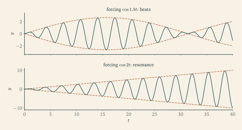
The two formulas are consistent. For fixed \(t\) , as \(\omega\to\omega_0\) the factor \(\sin\frac{(\omega_0-\omega)t}{2}\) is approximately \(\frac{(\omega_0-\omega)t}{2}\) and \(\omega_0^2-\omega^2=(\omega_0-\omega)(\omega_0+\omega)\) , so the beat solution tends to \(\frac{F}{2\omega_0}t\sin\omega_0t\) . Pure resonance is a beat of infinite length. The unbounded growth is an idealization: real oscillators have some damping, and real springs leave the linear regime. That is the subject of the next section.
5.5 Damped forcing: gain and phase lag
With damping, \(my''+cy'+ky=F_0\cos\omega t\) with \(m,c,k>0\) , the picture changes in two ways: the natural motions die out, and the response to forcing stays bounded at every frequency.
The characteristic polynomial is \(P(r)=mr^2+cr+k\) . Its roots have negative real parts, since their sum \(-c/m\) is negative and their product \(k/m\) is positive. In particular \(i\omega\) is never a root, and Theorem 5.2(a) always applies:
Write the complex number \(P(i\omega)\) in polar form, \(P(i\omega)=\lvert P(i\omega)\rvert e^{i\phi}\) . Its imaginary part \(c\omega\) is positive for \(\omega>0\) , so \(0<\phi<\pi\) . Taking the real part of \(z_p\) :
Theorem 5.4 (steady-state response). Let \(m,c,k>0\) and \(\omega>0\) . The equation \(my''+cy'+ky=F_0\cos\omega t\) has the particular solution
where \(\phi(\omega)\in(0,\pi)\) is the angle of the complex number \((k-m\omega^2)+ic\omega\) . Every solution of the equation is \(y_p\) plus a solution of the homogeneous equation, and the latter tends to \(0\) as \(t\to\infty\) . Hence every solution approaches \(y_p\) , and \(y_p\) is the only solution that has the period \(2\pi/\omega\) of the forcing.
Proof. The formula is the real part of \(F_0e^{i\omega t}/P(i\omega)=F_0\lvert P(i\omega)\rvert^{-1}e^{i(\omega t-\phi)}\) . By Theorem 5.1 every solution is \(y_p+y_h\) . By Theorem 4.6 \(y_h\) is a combination of functions \(e^{r_1t}\) , \(e^{r_2t}\) , \(te^{rt}\) , or \(e^{\lambda t}\cos\mu t\) , \(e^{\lambda t}\sin\mu t\) in which all exponents have negative real part, so \(y_h\to0\) . If a solution \(y_p+y_h\) had period \(2\pi/\omega\) , then so would \(y_h\) , and a periodic function that tends to \(0\) is identically zero.
The function \(y_p\) is the steady state and \(y_h\) the transient. The transient carries the initial conditions and disappears; the steady state depends only on the forcing. \(G(\omega)\) is the gain, the amplitude of the response per unit amplitude of force, and \(\phi(\omega)\) is the phase lag, with \(\tan\phi=c\omega/(k-m\omega^2)\) when \(k\ne m\omega^2\) .
Three regimes can be read from \(P(i\omega)=(k-m\omega^2)+ic\omega\) . For slow forcing, \(\omega\to0\) , it is nearly the real number \(k\) : \(G\to1/k\) and \(\phi\to0\) , so the mass follows the force as a static spring would. At \(\omega=\omega_0=\sqrt{k/m}\) it is purely imaginary, \(ic\omega_0\) : \(G=1/(c\omega_0)\) and \(\phi=\pi/2\) exactly, whatever the damping. For fast forcing it is dominated by \(-m\omega^2\) : \(G\approx1/(m\omega^2)\to0\) and \(\phi\to\pi\) , so the mass barely moves, and moves opposite to the force.
Proposition 5.5 (practical resonance). Let \(\omega_0^2=k/m\) and \(\omega_d^2=\omega_0^2-c^2/(4m^2)\) . If \(c^2<2mk\) , the gain \(G\) has a unique maximum on \(\omega\ge0\) , at
If \(c^2\ge2mk\) , the gain is strictly decreasing on \(\omega\ge0\) and its largest value is \(G(0)=1/k\) .
Proof. Maximizing \(G\) is minimizing \(D=(k-m\omega^2)^2+c^2\omega^2\) . As a function of \(u=\omega^2\ge0\) this is the quadratic \(D=m^2u^2+(c^2-2mk)u+k^2\) , which opens upward with vertex at \(u^{*}=(2mk-c^2)/(2m^2)\) . If \(c^2<2mk\) then \(u^{*}>0\) and the minimum over \(u\ge0\) is at \(u^{*}=\omega_0^2-c^2/(2m^2)\) , with value
If \(c^2\ge2mk\) then \(u^{*}\le0\) , so \(D\) is increasing on \(u\ge0\) and smallest at \(u=0\) , where \(D=k^2\) .
The peak is at a frequency slightly below \(\omega_0\) , and below the frequency \(\omega_d\) of the free damped oscillation too: \(\omega_r<\omega_d<\omega_0\) . For light damping the three nearly coincide and the peak gain is close to \(1/(c\omega_0)\) , inversely proportional to the damping. As \(c\to0\) the peak becomes infinite, which is the pure resonance of Section 5.4.
Example 5.6: A resonance curve in numbers
Take \(m=1\) , \(k=4\) , \(c=1\) , so \(\omega_0=2\) and \(c^2=1<2mk=8\) .
Peak. \(\omega_r=\sqrt{4-\tfrac12}=\sqrt{3.5}\approx1.871\) and \(\omega_d=\sqrt{4-\tfrac14}\approx1.936\) , so the peak gain is \(1/(c\,\omega_d)\approx0.516\) . The static gain is \(G(0)=1/k=0.25\) and the gain at the natural frequency is \(G(2)=1/(c\,\omega_0)=0.5\) . Forcing near \(\omega_r\) produces twice the displacement that the same force applied steadily would.
A specific input. For \(y''+y'+4y=3\cos t\) : \(P(i)=(4-1)+i=3+i\) , with \(\lvert3+i\rvert=\sqrt{10}\) and angle \(\phi=\arctan\tfrac13\approx0.322\) . The steady state is
or in rectangular form \(\operatorname{Re}\dfrac{3e^{it}}{3+i}=\dfrac{9\cos t+3\sin t}{10}\) .
Heavier damping. With \(c=3\) we have \(c^2=9\ge8\) and there is no resonance peak at all: the gain falls from \(0.25\) monotonically. With \(c=2\) the peak is at \(\omega_r=\sqrt2\approx1.414\) with gain \(1/(2\sqrt3)\approx0.289\) , barely above the static value.
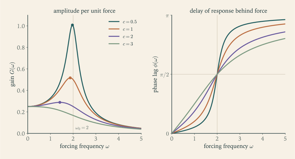
Figure 5.2 is the practical summary of this chapter. To avoid large vibrations, keep forcing frequencies away from the peak or add damping; to detect a weak signal of known frequency, as a radio tuner does, use a lightly damped system whose peak sits on that frequency. In both cases the transient must be allowed to die out first, and for light damping it dies slowly, at the rate \(e^{-ct/(2m)}\) .
Example 5.7: From rest to the steady state
Solve \(y''+2y'+5y=4\cos2t\) with \(y(0)=0\) , \(y'(0)=0\) : the oscillator of Example 5.2, switched on at rest.
By Theorem 5.1 and Example 5.2, \(y=y_p+e^{-t}(c_1\cos2t+c_2\sin2t)\) with \(y_p=\tfrac4{17}\cos2t+\tfrac{16}{17}\sin2t\) . The condition \(y(0)=0\) gives \(c_1=-\tfrac4{17}\) . Since \(y_p'(0)=\tfrac{32}{17}\) and the derivative of the second part at \(t=0\) is \(-c_1+2c_2\) , the condition \(y'(0)=0\) gives \(2c_2=c_1-\tfrac{32}{17}=-\tfrac{36}{17}\) , so \(c_2=-\tfrac{18}{17}\) :
The transient has amplitude \(\tfrac1{17}\sqrt{4^2+18^2}\,e^{-t}\approx1.085\,e^{-t}\) . At the start it is larger than the steady amplitude \(0.970\) , because it has to cancel both the value and the slope of the steady state at \(t=0\) . It drops below one percent of the steady amplitude when \(e^{-t}<0.0097/1.085\) , that is, after \(t\approx4.72\) , which is one and a half periods of the forcing. In numbers: at \(t=1\) the solution is \(0.440\) while the steady state is \(0.758\) ; at \(t=5\) they are \(-0.704\) and \(-0.709\) .
The example separates two questions that are easily run together. How large is the eventual response? That is answered by \(P(i\omega)\) alone. How long until the eventual response is what one sees? That is answered by the real parts of the characteristic roots, here \(-1\) . A lightly damped system has a tall resonance peak and, for the same reason, a long memory of how it was started.
Throughout this chapter the forcing was a smooth elementary function. Switches, pulses, and hammer blows are not, and the next chapter introduces a transform that handles them and makes the gain function \(1/P\) its central object.
Exercises
-
Solve \(y''+3y'+2y=10e^{3t}\) with \(y(0)=0\) , \(y'(0)=0\) , using Theorem 5.2 for the particular solution.
Answer
\(P(r)=r^2+3r+2\) , \(P(3)=20\) , so \(y_p=\tfrac12e^{3t}\) . With \(y=\tfrac12e^{3t}+c_1e^{-t}+c_2e^{-2t}\) the data give \(c_1+c_2=-\tfrac12\) and \(-c_1-2c_2=-\tfrac32\) , so \(c_2=2\) , \(c_1=-\tfrac52\) : \(y=\tfrac12e^{3t}-\tfrac52e^{-t}+2e^{-2t}\) .
-
Find the general solution of \(y''+3y'+2y=e^{-t}\) , explaining which case of Theorem 5.2 applies and why a trial of the form \(Ae^{-t}\) cannot work.
Answer
\(P(-1)=0\) and \(P'(-1)=2(-1)+3=1\ne0\) , so case (b): \(y_p=te^{-t}\) , and \(y=te^{-t}+c_1e^{-t}+c_2e^{-2t}\) . The trial \(Ae^{-t}\) fails because \(e^{-t}\) solves the homogeneous equation, so \(L[Ae^{-t}]=0\) for every \(A\) .
-
Find the general solution of \(y''+4y=8t^2\) by undetermined coefficients, and explain why the trial must include terms of lower degree even though the forcing has only one term.
Answer
Trial \(At^2+Bt+C\) : \(L[y]=2A+4At^2+4Bt+4C=8t^2\) gives \(A=2\) , \(B=0\) , \(C=-1\) . So \(y=2t^2-1+c_1\cos2t+c_2\sin2t\) . The lower-degree terms are needed because differentiating \(t^2\) twice produces a constant, which must be cancelled.
-
Use complex replacement to find a particular solution of \(y''+2y'+2y=5\cos t\) , and write it in the form \(R\cos(t-\phi)\) with numerical values of \(R\) and \(\phi\) .
Solution
Replace \(5\cos t\) by \(5e^{it}\) . The characteristic polynomial is \(P(r)=r^2+2r+2\) , and
\[ P(i)=-1+2i+2=1+2i\ne0 . \]By Theorem 5.2(a) a complex solution is
\[ z_p=\frac{5e^{it}}{1+2i}=\frac{5\,(1-2i)}{5}\,e^{it}=(1-2i)(\cos t+i\sin t). \]Its real part is the required particular solution:
\[ y_p=\cos t+2\sin t . \]For the amplitude-phase form, \(R=\sqrt{1^2+2^2}=\sqrt5\approx2.236\) , and \(\phi\) is the angle of \(1+2i\) , namely \(\phi=\arctan2\approx1.107\) . So \(y_p=\sqrt5\cos(t-1.107)\) . Equivalently, \(1+2i=\sqrt5e^{i\phi}\) gives \(z_p=\sqrt5e^{i(t-\phi)}\) directly. The gain is \(\sqrt5/5\approx0.447\) and the response lags the input by about \(63\) degrees.
-
Solve \(y''+4y=\sin2t\) with \(y(0)=0\) , \(y'(0)=0\) , giving the correct trial solution first, and describe the long-term behaviour of the solution.
Solution
The characteristic roots of \(y''+4y=0\) are \(\pm2i\) , and the forcing \(\sin2t\) has exponent \(2i\) , a simple root. So the trial is \(t\,(A\cos2t+B\sin2t)\) , not \(A\cos2t+B\sin2t\) .
The coefficients follow from Theorem 5.2(b). With \(P(r)=r^2+4\) , \(P'(2i)=4i\) , the function \(z=\dfrac{te^{2it}}{4i}\) satisfies \(L[z]=e^{2it}\) . Since \(\sin2t\) is the imaginary part of \(e^{2it}\) ,
\[ y_p=\operatorname{Im}\frac{t\,(\cos2t+i\sin2t)}{4i}=\operatorname{Im}\Bigl(-\frac{it}{4}(\cos2t+i\sin2t)\Bigr)=-\frac t4\cos2t . \]The general solution is \(y=-\tfrac t4\cos2t+c_1\cos2t+c_2\sin2t\) . From \(y(0)=0\) , \(c_1=0\) . Then \(y'(0)=-\tfrac14+2c_2=0\) gives \(c_2=\tfrac18\) :
\[ y=\tfrac18\sin2t-\tfrac t4\cos2t . \]The first term is bounded; the second oscillates with amplitude \(t/4\) , which grows without limit. This is pure resonance: the forcing frequency equals the natural frequency and there is no damping.
-
For \(y''-4y'+4y=g(t)\) write the form of the trial particular solution, without finding the coefficients, when (a) \(g=e^{2t}\) ; (b) \(g=te^{2t}+\cos t\) ; (c) \(g=e^{2t}\sin t\) ; (d) \(g=t^2+e^{-2t}\) .
Answer
The characteristic polynomial is \((r-2)^2\) . (a) \(At^2e^{2t}\) . (b) \(t^2(At+B)e^{2t}+C\cos t+D\sin t\) . (c) \(e^{2t}(A\cos t+B\sin t)\) , since \(2+i\) is not a root. (d) \(At^2+Bt+C+De^{-2t}\) .
-
Use variation of parameters to find a particular solution of \(y''+y=\tan t\) on \((-\pi/2,\pi/2)\) , and verify it by substitution.
Solution
Take \(y_1=\cos t\) , \(y_2=\sin t\) , \(W=1\) , and \(g=\tan t\) , continuous on the interval. Theorem 5.3 gives
\[ u_1'=-\sin t\tan t=-\frac{\sin^2t}{\cos t}=\cos t-\sec t,\qquad u_2'=\cos t\tan t=\sin t . \]Integrating, \(u_1=\sin t-\ln(\sec t+\tan t)\) , where \(\sec t+\tan t>0\) on \((-\pi/2,\pi/2)\) , and \(u_2=-\cos t\) . Hence
\[ y_p=\cos t\bigl(\sin t-\ln(\sec t+\tan t)\bigr)-\cos t\sin t=-\cos t\,\ln(\sec t+\tan t). \]The terms \(\pm\cos t\sin t\) cancel, which is typical: any multiple of \(y_1\) or \(y_2\) produced by the constants of integration may be discarded, and here part of \(u_1y_1\) is absorbed by \(u_2y_2\) .
Verification. Let \(\ell=\ln(\sec t+\tan t)\) , so \(\ell'=\sec t\) . Then \(y_p=-\ell\cos t\) , \(y_p'=\ell\sin t-1\) , and \(y_p''=\ell\cos t+\sec t\sin t=\ell\cos t+\tan t\) . Adding, \(y_p''+y_p=\tan t\) . The solution is valid on \((-\pi/2,\pi/2)\) and, unlike the forcing, stays bounded as \(t\) approaches the ends of the interval, because \(\cos t\,\ln(\sec t+\tan t)\to0\) there.
-
The functions \(t\) and \(t^2\) are solutions of \(t^2y''-2ty'+2y=0\) for \(t>0\) (Example 4.1). Use variation of parameters to solve \(t^2y''-2ty'+2y=t^3\) , taking care to identify \(g\) correctly, and verify the result.
Solution
Theorem 5.3 is stated for the normal form. Dividing by \(t^2\) ,
\[ y''-\frac2t\,y'+\frac2{t^2}\,y=t , \]so \(g=t\) , not \(t^3\) . With \(y_1=t\) , \(y_2=t^2\) , the Wronskian is \(W=t^2\) (Example 4.1). Then
\[ u_1'=-\frac{y_2g}{W}=-\frac{t^2\cdot t}{t^2}=-t,\qquad u_2'=\frac{y_1g}{W}=\frac{t\cdot t}{t^2}=1 , \]so \(u_1=-\tfrac12t^2\) , \(u_2=t\) , and
\[ y_p=-\tfrac12t^2\cdot t+t\cdot t^2=\tfrac12t^3 . \]Verification in the original equation: \(y_p'=\tfrac32t^2\) , \(y_p''=3t\) , and \(t^2(3t)-2t\bigl(\tfrac32t^2\bigr)+2\bigl(\tfrac12t^3\bigr)=3t^3-3t^3+t^3=t^3\) . The general solution for \(t>0\) is \(y=\tfrac12t^3+c_1t+c_2t^2\) . Had \(g=t^3\) been used, the result would have been \(\tfrac1{12}t^5\) , which does not satisfy the equation.
-
A student says: “Resonance means the forcing frequency equals the natural frequency, so for \(y''+2y'+4y=\cos\omega t\) the steady-state amplitude is largest at \(\omega=2\) .” Compute the gain at \(\omega=2\) and at the true maximizing frequency, and explain the error.
Solution
Here \(m=1\) , \(c=2\) , \(k=4\) , so \(\omega_0=2\) and the gain is \(G(\omega)=1/\sqrt{(4-\omega^2)^2+4\omega^2}\) .
At \(\omega=2\) : \(G(2)=1/\sqrt{0+16}=0.25\) .
By Proposition 5.5, since \(c^2=4<2mk=8\) , the maximum is at \(\omega_r=\sqrt{\omega_0^2-c^2/(2m^2)}=\sqrt{4-2}=\sqrt2\approx1.414\) , and \(\omega_d=\sqrt{4-1}=\sqrt3\) , so
\[ G(\omega_r)=\frac{1}{c\,\omega_d}=\frac{1}{2\sqrt3}\approx0.289 . \]Direct check: \((4-2)^2+4\cdot2=12\) and \(1/\sqrt{12}\approx0.289\) . So the amplitude at \(\omega=\sqrt2\) exceeds the amplitude at \(\omega=2\) by about fifteen percent.
The student’s statement is correct for an undamped oscillator, where the response is unbounded exactly at \(\omega=\omega_0\) . With damping, the amplitude is \(1/\lvert P(i\omega)\rvert\) , and \(\lvert P(i\omega)\rvert^2=(k-m\omega^2)^2+c^2\omega^2\) is not minimized where the first term vanishes, because lowering \(\omega\) slightly below \(\omega_0\) reduces the second term by more than it increases the first. What does happen exactly at \(\omega_0\) is that the phase lag equals \(\pi/2\) .
-
For \(y''+9y=\cos3.2t\) with \(y(0)=0\) , \(y'(0)=0\) , write the solution as a product of two sines, and give the maximum amplitude and the time between successive moments at which the envelope vanishes.
Answer
\(\omega^2-\omega_0^2=10.24-9=1.24\) , so \(y=\dfrac{\cos3t-\cos3.2t}{1.24}=\dfrac{2}{1.24}\sin(0.1t)\sin(3.1t)\approx1.613\sin(0.1t)\sin(3.1t)\) . The maximum amplitude is \(1.613\) , and the envelope vanishes every \(2\pi/0.2\approx31.4\) time units.
-
A \(2\ \mathrm{kg}\) mass on a spring of stiffness \(8\ \mathrm{N/m}\) , with no damping and initially at rest, is driven by the force \(4\cos2t\) newtons. Find the displacement and the time at which the amplitude envelope first reaches \(3\ \mathrm{m}\) .
Answer
\(2y''+8y=4\cos2t\) , that is \(y''+4y=2\cos2t\) , with \(\omega_0=2\) : pure resonance. \(y=\dfrac{F}{2\omega_0}t\sin\omega_0t=\tfrac12t\sin2t\) metres. The envelope \(t/2\) reaches \(3\ \mathrm{m}\) at \(t=6\ \mathrm{s}\) .
-
Prove that for each fixed \(t\) the beat solution \(\dfrac{F}{\omega_0^2-\omega^2}(\cos\omega t-\cos\omega_0t)\) tends to \(\dfrac{F}{2\omega_0}t\sin\omega_0t\) as \(\omega\to\omega_0\) , by treating the expression as a difference quotient in \(\omega\) .
Solution
Fix \(t\) and define \(h(\omega)=\cos\omega t\) , a differentiable function of \(\omega\) with \(h'(\omega)=-t\sin\omega t\) . The beat solution is
\[ \frac{F\,\bigl(h(\omega)-h(\omega_0)\bigr)}{\omega_0^2-\omega^2}=-\frac{F}{\omega_0+\omega}\cdot\frac{h(\omega)-h(\omega_0)}{\omega-\omega_0}, \]using \(\omega_0^2-\omega^2=-(\omega-\omega_0)(\omega+\omega_0)\) . As \(\omega\to\omega_0\) the second factor is a difference quotient and tends to the derivative \(h'(\omega_0)=-t\sin\omega_0t\) , while the first factor tends to \(-F/(2\omega_0)\) . The product tends to
\[ -\frac{F}{2\omega_0}\cdot\bigl(-t\sin\omega_0t\bigr)=\frac{F}{2\omega_0}\,t\sin\omega_0t . \]So the resonant solution is the pointwise limit of the off-resonance solutions. The convergence is not uniform in \(t\) : for any \(\omega\ne\omega_0\) the beat solution is bounded, while the limit is not, so the approximation is good only for times short compared with the beat length \(2\pi/\lvert\omega_0-\omega\rvert\) .
-
For \(y''+2y'+10y=12\cos\omega t\) find the frequency \(\omega_r\) of practical resonance, the largest steady-state amplitude, and the steady-state amplitude under very slow forcing.
Solution
Here \(m=1\) , \(c=2\) , \(k=10\) , \(F_0=12\) , so \(\omega_0^2=10\) . Since \(c^2=4<2mk=20\) , Proposition 5.5 gives a resonance peak at
\[ \omega_r=\sqrt{\omega_0^2-\frac{c^2}{2m^2}}=\sqrt{10-2}=\sqrt8\approx2.828 . \]The damped natural frequency is \(\omega_d=\sqrt{10-1}=3\) , so the peak gain is \(G(\omega_r)=1/(c\,\omega_d)=1/6\) , and the largest steady-state amplitude is \(F_0G(\omega_r)=12/6=2\) . As a check, \((10-8)^2+4\cdot8=36\) and \(1/\sqrt{36}=1/6\) .
For very slow forcing, \(\omega\to0\) , the gain tends to \(G(0)=1/k=0.1\) and the amplitude to \(12/10=1.2\) , the static deflection under a constant force of \(12\) . Resonance therefore multiplies the static response by \(2/1.2\approx1.67\) . At the natural frequency itself the amplitude is \(12/(c\,\omega_0)=12/(2\sqrt{10})\approx1.90\) , slightly below the peak.
-
Show that at \(\omega=\omega_0\) the steady state of \(my''+cy'+ky=F_0\cos\omega t\) is \(y_p=\dfrac{F_0}{c\,\omega_0}\sin\omega_0t\) , and deduce that the velocity \(y_p'\) is then exactly in phase with the force. Explain why this makes the power delivered by the force as large as possible.
Hint
At \(\omega=\omega_0\) , \(P(i\omega_0)=ic\,\omega_0\) , so \(z_p=F_0e^{i\omega_0t}/(ic\,\omega_0)\) ; take the real part. Power is force times velocity; average \(\cos\omega_0t\cdot\cos(\omega_0t-\theta)\) over a period and see which \(\theta\) makes it largest.
-
Let \(m,c,k>0\) and let \(F\) be continuous on \([0,\infty)\) . Using the results of Chapter 4, prove that any two solutions of \(my''+cy'+ky=F(t)\) differ by a function that tends to \(0\) as \(t\to\infty\) , and state what this means for the role of initial conditions.
Hint
The difference of two solutions solves the homogeneous equation. Use Theorem 4.6 and the signs of the real parts of the roots of \(mr^2+cr+k\) .
-
An instrument of mass \(1\ \mathrm{kg}\) is mounted on a spring of stiffness \(100\ \mathrm{N/m}\) . Find the smallest damping coefficient for which a force \(F_0\cos\omega_0t\) at the natural frequency produces a steady amplitude no more than twice the static deflection \(F_0/k\) .
Hint
At \(\omega_0\) the gain is \(1/(c\,\omega_0)\) and the static deflection per unit force is \(1/k\) . The condition \(1/(c\,\omega_0)\le2/k\) gives \(c\ge k/(2\omega_0)\) ; here \(\omega_0=10\ \mathrm{rad/s}\) and the answer is \(5\ \mathrm{N\,s/m}\) .
-
Find a particular solution of \(y''+2y'+5y=4\cos2t+10\) using Example 5.2 and superposition of forcings, and state the average value about which the steady state oscillates.
Answer
For the constant forcing \(10\) , \(y=2\) works since \(5\cdot2=10\) . By superposition \(y_p=\tfrac4{17}\cos2t+\tfrac{16}{17}\sin2t+2\) , which oscillates about the average value \(2\) .
-
Use the single-integral form of variation of parameters to show that \(y(t)=\dfrac{1}{\omega_0}\displaystyle\int_0^t\sin\bigl(\omega_0(t-s)\bigr)\,g(s)\,ds\) solves \(y''+\omega_0^2y=g\) with \(y(0)=y'(0)=0\) , and evaluate it for \(g=1\) .
Solution
For \(y''+\omega_0^2y=0\) take \(y_1=\cos\omega_0t\) , \(y_2=\sin\omega_0t\) , with Wronskian \(W=\omega_0\) . The kernel in the single-integral form of Theorem 5.3 is
\[ \frac{y_1(s)y_2(t)-y_1(t)y_2(s)}{W(s)}=\frac{\cos\omega_0s\,\sin\omega_0t-\cos\omega_0t\,\sin\omega_0s}{\omega_0}=\frac{\sin\bigl(\omega_0(t-s)\bigr)}{\omega_0}, \]by the subtraction formula for the sine. With \(t_0=0\) this gives the stated \(y(t)\) , and by the remark after Theorem 5.3 it satisfies \(y(0)=0\) , \(y'(0)=0\) .
One can also verify directly. Differentiating under the integral sign, the boundary term is \(\sin(0)\,g(t)/\omega_0=0\) , so \(y'(t)=\int_0^t\cos(\omega_0(t-s))\,g(s)\,ds\) . Differentiating again, the boundary term is now \(\cos(0)\,g(t)=g(t)\) , and \(y''(t)=g(t)-\omega_0\int_0^t\sin(\omega_0(t-s))\,g(s)\,ds=g(t)-\omega_0^2y(t)\) .
For \(g=1\) :
\[ y(t)=\frac1{\omega_0}\int_0^t\sin\bigl(\omega_0(t-s)\bigr)\,ds=\frac{1-\cos\omega_0t}{\omega_0^2}. \]A constant force switched on at \(t=0\) makes the mass oscillate about the new equilibrium \(1/\omega_0^2\) , overshooting to twice that value.