A thermostat turns a heater on at \(t=1\) and off at \(t=3\) . The room temperature, measured from its resting value, obeys \(y'+y=f(t)\) with \(f\) equal to \(1\) while the heater is on and \(0\) otherwise. The methods of Chapter 2 can solve this, three times over: once on each of the intervals \([0,1)\) , \([1,3)\) , \([3,\infty)\) , with the final value on one interval supplying the initial value on the next. For a second-order equation with several switches the bookkeeping multiplies, and for a hammer blow, a force that is enormous for an instant and zero otherwise, it is not even clear what function to write on the right-hand side.
The Laplace transform handles all of this in one calculation. It replaces a function of time by a function of a new variable \(s\) , and under that replacement differentiation turns into multiplication by \(s\) , a delay turns into multiplication by an exponential, and initial values enter automatically. A linear differential equation with constant coefficients becomes an algebraic equation. The price is a table of transforms and some care about when the rules apply, and that care is where most errors with the method are made.
6.1 The transform and when it exists
Definition 6.1 (Laplace transform). Let \(f\) be defined for \(t\ge0\) . Its Laplace transform is the function
defined for those real \(s\) for which the limit exists.
The transform looks only at \(t\ge0\) ; it is designed for problems that start at time zero. Lower-case letters will denote functions of \(t\) and the corresponding capitals their transforms.
For the integral to make sense \(f\) must be integrable on bounded intervals, and for it to converge \(f\) must not grow too fast.
Definition 6.2 (piecewise continuity and exponential order). A function \(f\) on \([0,\infty)\) is piecewise continuous if on every bounded interval it is continuous except at finitely many points, at each of which it has finite one-sided limits. It is of exponential order \(c\) if there are constants \(M\) and \(c\) with \(\lvert f(t)\rvert\le Me^{ct}\) for all \(t\ge0\) .
Theorem 6.3 (existence of the transform). If \(f\) is piecewise continuous on \([0,\infty)\) and of exponential order \(c\) , then \(F(s)\) exists for every \(s>c\) , and
In particular \(F(s)\to0\) as \(s\to\infty\) .
Proof. For \(s>c\) , \(\lvert e^{-st}f(t)\rvert\le Me^{-(s-c)t}\) , and \(\int_0^{\infty}Me^{-(s-c)t}\,dt=M/(s-c)\) converges. An improper integral whose integrand is piecewise continuous and bounded in absolute value by an integrable function converges, and its absolute value is at most the integral of the bound.
Polynomials, exponentials, sines and cosines, and all their sums and products are of exponential order. The function \(e^{t^2}\) is not, and it has no Laplace transform for any \(s\) . The last sentence of the theorem is a useful test: a function such as \(s/(s+1)\) , which tends to \(1\) , is not the transform of any piecewise continuous function of exponential order.
The transform is linear, \(\mathcal L\{\alpha f+\beta g\}=\alpha F+\beta G\) wherever both exist, because the integral is.
Example 6.1: The basic transforms from the definition
A constant. \(\mathcal L\{1\}=\displaystyle\int_0^{\infty}e^{-st}\,dt=\frac1s\) for \(s>0\) .
An exponential. For real or complex \(a\) , \(\mathcal L\{e^{at}\}=\displaystyle\int_0^{\infty}e^{-(s-a)t}\,dt=\frac{1}{s-a}\) , valid when \(s\) exceeds the real part of \(a\) .
Sine and cosine. Take \(a=ib\) in the previous line: \(\mathcal L\{e^{ibt}\}=\dfrac{1}{s-ib}=\dfrac{s+ib}{s^2+b^2}\) for \(s>0\) . Since \(e^{ibt}=\cos bt+i\sin bt\) , separating real and imaginary parts gives
A power. Integrating by parts, for \(s>0\) ,
and repeating the argument gives \(\mathcal L\{t^n\}=n!/s^{n+1}\) .
To use the transform for solving equations one must be able to go back from \(F\) to \(f\) . That is legitimate because of the following fact, quoted here without proof.
Theorem 6.4 (uniqueness of the inverse transform). If \(f\) and \(g\) are piecewise continuous, of exponential order, and \(F(s)=G(s)\) for all sufficiently large \(s\) , then \(f(t)=g(t)\) at every \(t\ge0\) at which both are continuous.
So a continuous function is determined by its transform, and one may write \(f=\mathcal L^{-1}\{F\}\) . In practice the inverse is found by rearranging \(F\) into pieces that appear in a table.
6.2 Derivatives become multiplication
Theorem 6.5 (transform of a derivative). Let \(f\) be continuous on \([0,\infty)\) and of exponential order \(c\) , with \(f'\) piecewise continuous. Then for \(s>c\) ,
If also \(f'\) is continuous and of exponential order \(c\) and \(f''\) is piecewise continuous, then \(\mathcal L\{f''\}(s)=s^2F(s)-sf(0)-f'(0)\) .
Proof. On an interval \([0,T]\) , split at the finitely many points where \(f'\) is discontinuous and integrate by parts on each piece. Because \(f\) is continuous, the boundary terms at interior points cancel, leaving
For \(s>c\) , \(\lvert e^{-sT}f(T)\rvert\le Me^{-(s-c)T}\to0\) as \(T\to\infty\) , and the last integral tends to \(F(s)\) . For the second formula apply the first to \(f'\) : \(\mathcal L\{f''\}=s\,\mathcal L\{f'\}-f'(0)=s\bigl(sF-f(0)\bigr)-f'(0)\) .
The continuity of \(f\) is essential: at a jump of \(f\) the interior boundary terms would not cancel. The initial values \(f(0)\) and \(f'(0)\) appear of their own accord, and this is what makes the transform suited to initial value problems.
Apply the theorem to \(ay''+by'+cy=g(t)\) with \(y(0)=y_0\) , \(y'(0)=v_0\) . Transforming both sides,
The characteristic polynomial of Chapter 4 appears as the denominator. The first term is the response to the forcing from rest; the second is the free response to the initial data. The method assumes that the solution has a transform. For constant coefficients and forcing of exponential order it does, and in any case the function obtained at the end can be checked by substitution.
A second rule supplies the transforms needed to invert such quotients.
Theorem 6.6 (first shifting rule). If \(F(s)=\mathcal L\{f\}(s)\) exists for \(s>c\) , then \(\mathcal L\{e^{at}f(t)\}(s)=F(s-a)\) for \(s>c+a\) .
Proof. \(\displaystyle\int_0^{\infty}e^{-st}e^{at}f(t)\,dt=\int_0^{\infty}e^{-(s-a)t}f(t)\,dt=F(s-a)\) .
Hence \(\mathcal L\{t^ne^{at}\}=\dfrac{n!}{(s-a)^{n+1}}\) , \(\mathcal L\{e^{at}\cos bt\}=\dfrac{s-a}{(s-a)^2+b^2}\) , and \(\mathcal L\{e^{at}\sin bt\}=\dfrac{b}{(s-a)^2+b^2}\) . These, read from right to left, are exactly the pieces that a partial-fraction decomposition produces: a real root of \(P\) of multiplicity \(k\) gives terms \(1/(s-a)^j\) , and a pair of complex roots gives a quadratic that is put in the form \((s-a)^2+b^2\) by completing the square.
| Function \(f(t)\) | Transform \(F(s)\) |
|---|---|
| \(1\) | \(1/s\) |
| \(t^n\) | \(n!/s^{n+1}\) |
| \(e^{at}\) | \(1/(s-a)\) |
| \(\cos bt\) | \(s/(s^2+b^2)\) |
| \(\sin bt\) | \(b/(s^2+b^2)\) |
| \(e^{at}f(t)\) | \(F(s-a)\) |
| \(f'(t)\) | \(sF(s)-f(0)\) |
| \(f''(t)\) | \(s^2F(s)-sf(0)-f'(0)\) |
| \(u(t-a)f(t-a)\) | \(e^{-as}F(s)\) |
| \((f*g)(t)\) | \(F(s)G(s)\) |
| \(\delta(t-a)\) | \(e^{-as}\) |
The last three rows are established in Sections 6.3 to 6.5.
Example 6.2: An initial value problem with real roots
Solve \(y''-3y'+2y=e^{3t}\) , \(y(0)=1\) , \(y'(0)=0\) .
Transforming: \((s^2Y-s)-3(sY-1)+2Y=\dfrac{1}{s-3}\) , so
Partial fractions, found by covering each factor in turn:
Adding and inverting term by term,
Check: \(y(0)=\tfrac52-2+\tfrac12=1\) and \(y'(0)=\tfrac52-4+\tfrac32=0\) . The term \(\tfrac12e^{3t}\) is the particular solution \(e^{3t}/P(3)\) of Theorem 5.2, and the other two terms are the complementary solution with its constants already fitted. No separate step for the initial conditions was needed.
Example 6.3: Complex roots and a step response
Solve \(y''+2y'+5y=5\) , \(y(0)=0\) , \(y'(0)=0\) : a damped oscillator at rest to which a constant force is suddenly applied.
Transforming, \((s^2+2s+5)Y=5/s\) . Write \(\dfrac{5}{s(s^2+2s+5)}=\dfrac As+\dfrac{Bs+C}{s^2+2s+5}\) . Multiplying out, \(5=A(s^2+2s+5)+(Bs+C)s\) , so \(A=1\) , \(B=-1\) , \(C=-2\) :
Completing the square has put the quadratic in shifted form, and the numerator has been split to match the cosine and sine entries. Therefore
The solution tends to the new equilibrium \(y=1\) . Its derivative is \(y'=\tfrac52e^{-t}\sin2t\) , which first vanishes at \(t=\pi/2\) , where \(y=1+e^{-\pi/2}\approx1.208\) : the oscillator overshoots its final position by about \(21\) percent.
Common mistake. Writing \(\mathcal L\{y'\}=sY\) and losing the initial value. For \(y'+2y=0\) , \(y(0)=3\) this gives \((s+2)Y=0\) , hence \(Y=0\) and \(y=0\) , which does not satisfy \(y(0)=3\) . The correct transform is \(sY-3+2Y=0\) , \(Y=3/(s+2)\) , \(y=3e^{-2t}\) . Write the full derivative rule, with every initial term, before doing any algebra.
6.3 Switches and delays
Definition 6.7 (unit step). For \(a\ge0\) the unit step function at \(a\) is
Multiplying by \(u(t-a)\) switches a function on at time \(a\) , and \(u(t-a)-u(t-b)\) is a pulse that is \(1\) on \([a,b)\) and \(0\) elsewhere. Any piecewise-defined forcing can be written with steps: a function equal to \(f_1\) before time \(a\) and \(f_2\) after it is \(f_1(t)+u(t-a)\bigl(f_2(t)-f_1(t)\bigr)\) .
Theorem 6.8 (second shifting rule). If \(F=\mathcal L\{f\}\) exists for \(s>c\) and \(a\ge0\) , then
Proof. The integrand vanishes for \(t<a\) , so the transform is \(\int_a^{\infty}e^{-st}f(t-a)\,dt\) . Substituting \(\tau=t-a\) gives \(\int_0^{\infty}e^{-s(\tau+a)}f(\tau)\,d\tau=e^{-as}F(s)\) .
In words: delaying a signal by \(a\) , with nothing before time \(a\) , multiplies its transform by \(e^{-as}\) . With \(f=1\) this gives \(\mathcal L\{u(t-a)\}=e^{-as}/s\) . Read backward, a factor \(e^{-as}\) in a transform means: invert the rest, then delay the result by \(a\) and switch it on at \(a\) .
Example 6.4: The thermostat
Solve \(y'+y=u(t-1)-u(t-3)\) , \(y(0)=0\) .
Transforming, \((s+1)Y=\dfrac{e^{-s}-e^{-3s}}{s}\) , so \(Y=(e^{-s}-e^{-3s})\,H(s)\) with \(H(s)=\dfrac{1}{s(s+1)}=\dfrac1s-\dfrac{1}{s+1}\) . The inverse of \(H\) is \(h(t)=1-e^{-t}\) , and by Theorem 6.8
Unpacking the steps: \(y=0\) for \(t<1\) ; \(y=1-e^{-(t-1)}\) for \(1\le t<3\) , rising toward \(1\) ; and for \(t\ge3\) ,
decaying from the value \(y(3)=1-e^{-2}\approx0.865\) reached when the heater switched off. At \(t=5\) , \(y=e^{-2}-e^{-4}\approx0.117\) . The solution is continuous at both switching times, while its derivative jumps there by \(+1\) and \(-1\) , as the equation \(y'=f-y\) demands. The single formula contains the three-interval calculation and the matching conditions.
Common mistake. Applying the shift rule to \(u(t-a)f(t)\) as though it were \(u(t-a)f(t-a)\) . The transform of \(u(t-1)\,t\) is not \(e^{-s}/s^2\) . The function multiplying the step must first be written in terms of \(t-a\) : \(t=(t-1)+1\) , so \(u(t-1)\,t=u(t-1)\bigl[(t-1)+1\bigr]\) and the transform is \(e^{-s}\bigl(1/s^2+1/s\bigr)\) .
Example 6.5: When the force is switched off matters
An undamped oscillator at rest is pushed with a constant unit force from \(t=0\) until \(t=T\) : \(y''+y=1-u(t-T)\) , \(y(0)=y'(0)=0\) .
Transforming, \((s^2+1)Y=\dfrac{1-e^{-Ts}}{s}\) . Since \(\dfrac{1}{s(s^2+1)}=\dfrac1s-\dfrac{s}{s^2+1}\) has inverse \(1-\cos t\) ,
For \(t\ge T\) this is \(y=\cos(t-T)-\cos t\) .
If \(T=\pi\) : \(\cos(t-\pi)=-\cos t\) , so \(y=-2\cos t\) for \(t\ge\pi\) . The oscillator is left swinging with amplitude \(2\) .
If \(T=2\pi\) : \(\cos(t-2\pi)=\cos t\) , so \(y=0\) for \(t\ge2\pi\) . The oscillator is left exactly at rest.
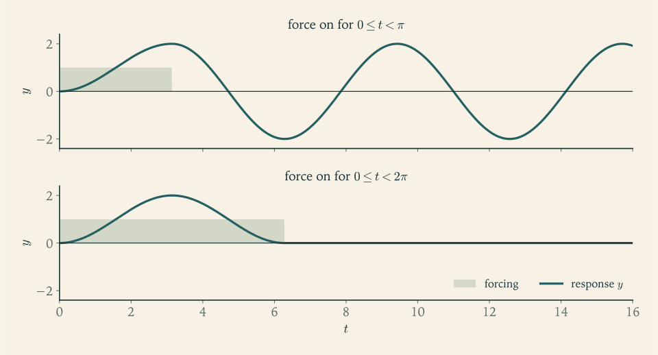
The explanation is in the first formula. While the force is on, the mass oscillates about the displaced equilibrium \(y=1\) , between \(0\) and \(2\) . At \(t=\pi\) it is at \(y=2\) with zero velocity, two units from the equilibrium \(y=0\) that governs once the force is removed. At \(t=2\pi\) it is at \(y=0\) with zero velocity, which is the rest state of the unforced system. This is the idea of Chapter 5 in another form: the effect of a force depends on its timing relative to the system’s own rhythm.
6.4 Convolution and the transfer function
The forced response from rest has transform \(G(s)/P(s)\) , a product of two transforms. The inverse of a product is not the product of the inverses; it is the following operation.
Definition 6.9 (convolution). The convolution of two piecewise continuous functions on \([0,\infty)\) is
The substitution \(\tau\mapsto t-\tau\) shows that \(f*g=g*f\) .
Theorem 6.10 (convolution theorem). If \(f\) and \(g\) are piecewise continuous and of exponential order \(c\) , then \(\mathcal L\{f*g\}(s)=F(s)\,G(s)\) for \(s>c\) .
Proof. Fix \(s>c\) and put \(k=s-c>0\) . Choose \(M\) so that \(\lvert f(t)\rvert\le Me^{ct}\) and \(\lvert g(t)\rvert\le Me^{ct}\) . For \(T>0\) write \(F_T=\int_0^Te^{-s\sigma}f(\sigma)\,d\sigma\) and \(G_T=\int_0^Te^{-s\tau}g(\tau)\,d\tau\) , so that \(F_T\to F(s)\) and \(G_T\to G(s)\) as \(T\to\infty\) .
A finite identity. The truncated transform of the convolution is an iterated integral over the triangle \(0\le\tau\le t\le T\) , and may be taken in either order:
For a continuous integrand the change of order is the theorem on iterated integrals from Multivariable Calculus (math.multivariable-calculus.fubini-continuous). Here the integrand is bounded and is continuous except along finitely many line segments, those on which \(f(t-\tau)\)
or \(g(\tau)\)
jumps. The extension of the theorem to such integrands, obtained by cutting the triangle along those segments, is the one step of this proof that is quoted and not proved. Substituting \(\sigma=t-\tau\)
in the inner integral on the right gives
The tail. If the upper limit \(T-\tau\) were \(T\) , the right side would be exactly \(F_TG_T\) . The difference is controlled by the exponential bounds, \(\lvert e^{-s\sigma}f(\sigma)\rvert\le Me^{-k\sigma}\) and \(\lvert e^{-s\tau}g(\tau)\rvert\le Me^{-k\tau}\) :
The right side tends to \(0\) as \(T\to\infty\) . Hence \(\int_0^Te^{-st}(f*g)(t)\,dt-F_TG_T\to0\) , and since \(F_TG_T\to F(s)G(s)\) , the transform of \(f*g\) exists and equals \(F(s)G(s)\) .
Now return to \(ay''+by'+cy=g(t)\) with zero initial data, for which \(Y=G/P\) .
Definition 6.11 (transfer function and weight function). For the operator \(L[y]=ay''+by'+cy\) , the transfer function is \(W(s)=1/P(s)\) , and the weight function \(w\) is its inverse transform. Equivalently, \(w\) is the solution of \(L[w]=0\) with \(w(0)=0\) , \(w'(0)=1/a\) .
The two descriptions agree: transforming \(L[w]=0\) with those data gives \(P(s)W-a\cdot\tfrac1a=0\) . By the convolution theorem, the solution from rest is
This is the single-integral formula found by variation of parameters in Section 5.3, now with its kernel identified. The response at time \(t\) adds up the forcing at each earlier time \(\tau\) , weighted by \(w(t-\tau)\) , a function of the elapsed time only. The system is completely described, as far as its response from rest is concerned, by the one function \(w\) , or equivalently by \(W\) . And evaluating the transfer function on the imaginary axis recovers Chapter 5: \(W(i\omega)=1/P(i\omega)\) is the complex number whose modulus is the gain and whose angle is minus the phase lag.
Example 6.6: A response computed two ways
Solve \(y''+y=t\) , \(y(0)=y'(0)=0\) .
By convolution. \(P(s)=s^2+1\) , so \(w(t)=\sin t\) , and
By partial fractions. \(Y=\dfrac{1}{s^2(s^2+1)}=\dfrac1{s^2}-\dfrac{1}{s^2+1}\) , so \(y=t-\sin t\) .
Check: \(y''+y=\sin t+t-\sin t=t\) , and \(y(0)=0\) , \(y'(0)=1-1=0\) .
Partial fractions make the form of a solution visible before any inversion is carried out. If \(Y(s)\) is a quotient of polynomials, each root \(a\) of its denominator, called a pole of \(Y\) , contributes terms \(t^je^{at}\) with \(j\) less than the multiplicity of the root, and a complex pair \(\lambda\pm i\mu\) contributes \(e^{\lambda t}\cos\mu t\) and \(e^{\lambda t}\sin\mu t\) with the same powers of \(t\) . So the solution decays if every pole has negative real part, oscillates without decaying if the poles of largest real part are simple and lie on the imaginary axis, and grows if a pole has positive real part or is repeated on the imaginary axis. For the forced response \(G(s)/P(s)\) the poles are those of the forcing together with the characteristic roots; the first kind produce the steady response and the second kind the transient. When a pole of the forcing coincides with a characteristic root the multiplicity goes up by one, and that extra power of \(t\) is resonance (Exercises 5 and 12).
6.5 Impulses
A hammer strikes a mass. The force is very large and lasts a very short time; what matters is its impulse, the integral of force over time, which equals the change in momentum. Model the blow at time \(a\) by a pulse of width \(\varepsilon\) and height \(1/\varepsilon\) , so that the impulse is \(1\) :
Its transform is \(\dfrac{e^{-as}}{s}\cdot\dfrac{1-e^{-\varepsilon s}}{\varepsilon}\) , and since \((1-e^{-\varepsilon s})/\varepsilon\to s\) as \(\varepsilon\to0\) , the transforms tend to \(e^{-as}\) . The pulses themselves have no limit among functions: they become infinitely tall and infinitely thin. But the responses to them do have a limit.
Proposition 6.12 (limit of pulse responses). Let \(w\) be the weight function of \(L[y]=ay''+by'+cy\) , and let \(y_\varepsilon\) be the solution of \(L[y]=d_\varepsilon(t-a)\) with \(y(0)=y'(0)=0\) . Then for every \(t\ne a\) ,
Proof. By the convolution formula \(y_\varepsilon(t)=\int_0^{t}w(t-\tau)\,d_\varepsilon(\tau-a)\,d\tau\) . If \(t<a\) the pulse has not begun and \(y_\varepsilon(t)=0\) . If \(t>a\) , then for all \(\varepsilon<t-a\) the pulse lies inside \([0,t]\) and
the average of the continuous function \(\tau\mapsto w(t-\tau)\) over an interval shrinking to the point \(a\) . Such averages converge to the value at the point, \(w(t-a)\) .
It is convenient to have a symbol for the idealized blow. One writes \(\delta(t-a)\) , the unit impulse or Dirac delta at time \(a\) , and uses it by two rules that the proposition justifies: its transform is \(\mathcal L\{\delta(t-a)\}=e^{-as}\) , and the solution of \(L[y]=\delta(t-a)\) from rest is \(u(t-a)w(t-a)\) . The symbol does not stand for a function; a rigorous theory treats it as a generalized function and is outside this book. Here it is shorthand for “the limit of the responses to ever shorter pulses of unit impulse”. The weight function is thus the response to a unit impulse at time \(0\) , and is also called the impulse response.
What an impulse does physically is visible in \(w\) : since \(w(0)=0\) and \(w'(0)=1/a\) , a unit impulse leaves the position unchanged and changes the velocity instantly by \(1/a\) . For a mass \(m\) , a blow of impulse \(J\) changes the velocity by \(J/m\) .
Example 6.7: A hammer blow
Solve \(y''+2y'+2y=\delta(t-1)\) , \(y(0)=y'(0)=0\) .
Transforming, \((s^2+2s+2)Y=e^{-s}\) , so \(Y=\dfrac{e^{-s}}{(s+1)^2+1}\) . The inverse of \(1/((s+1)^2+1)\) is \(w(t)=e^{-t}\sin t\) , and the factor \(e^{-s}\) delays it:
The system stays at rest until \(t=1\) , then moves off with velocity \(1\) and performs a damped oscillation. The largest displacement occurs where \(w'=e^{-\tau}(\cos\tau-\sin\tau)\) vanishes, at \(\tau=t-1=\pi/4\) , and equals \(e^{-\pi/4}\sin(\pi/4)\approx0.322\) .
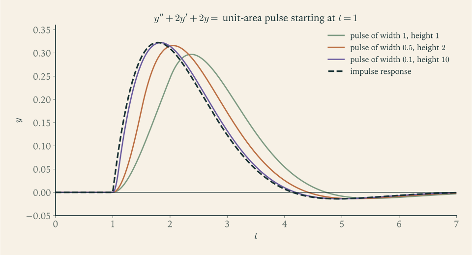
Figure 6.2 is Proposition 6.12 in a picture, and it carries a practical message. If a force acts for a time much shorter than the time scale on which the system itself changes, its detailed shape is irrelevant; only its impulse matters, and it may be replaced by a delta.
The Laplace transform is a tool for linear equations with constant coefficients. For variable coefficients the transformed equation is itself a differential equation, and for nonlinear equations the method does not apply at all. Within its domain it has done more than solve equations: it has shown that such a system is characterized by one function of \(s\) , the transfer function, whose poles are the characteristic roots. The next chapter generalizes in a different direction, from one unknown to many.
Exercises
-
Let \(f(t)=t\) for \(0\le t<1\) and \(f(t)=1\) for \(t\ge1\) . Compute \(\mathcal L\{f\}\) directly from the definition, then again by writing \(f\) with a unit step and using Theorem 6.8, and confirm that the two results agree.
Solution
From the definition. Split the integral at \(t=1\) :
\[ F(s)=\int_0^{1}te^{-st}\,dt+\int_1^{\infty}e^{-st}\,dt . \]Integrating by parts, \(\int_0^{1}te^{-st}\,dt=\Bigl[-\dfrac{t\,e^{-st}}{s}\Bigr]_0^{1}+\dfrac1s\int_0^{1}e^{-st}\,dt=-\dfrac{e^{-s}}{s}+\dfrac{1-e^{-s}}{s^2}\) . The second integral is \(e^{-s}/s\) for \(s>0\) . The terms \(\mp e^{-s}/s\) cancel, leaving
\[ F(s)=\frac{1-e^{-s}}{s^2}. \]With a step. The function is \(t\) until time \(1\) and then stops growing, so \(f(t)=t-u(t-1)(t-1)\) : after \(t=1\) the subtracted term removes exactly the growth beyond \(1\) . The second term has the form \(u(t-a)g(t-a)\) with \(g(t)=t\) , so Theorem 6.8 gives
\[ F(s)=\frac1{s^2}-\frac{e^{-s}}{s^2}, \]the same result. The step-function route needs no integration, only the correct expression of \(f\) in shifted form.
-
Use linearity, the table, and the shift in \(s\) to find the transforms of (a) \(3-2t+t^3\) ; (b) \(e^{-2t}\cos3t\) ; (c) \(t^2e^{4t}\) ; (d) \(\sin^2t\) .
Answer
(a) \(\dfrac3s-\dfrac2{s^2}+\dfrac6{s^4}\) . (b) \(\dfrac{s+2}{(s+2)^2+9}\) . (c) \(\dfrac{2}{(s-4)^3}\) . (d) Since \(\sin^2t=\tfrac12(1-\cos2t)\) : \(\dfrac1{2s}-\dfrac{s}{2(s^2+4)}=\dfrac{2}{s(s^2+4)}\) .
-
Find the inverse transforms of (a) \(\dfrac{3s+1}{s^2+4}\) ; (b) \(\dfrac{1}{s^2+4s+13}\) ; (c) \(\dfrac{s+3}{s^2-s-2}\) ; (d) \(\dfrac{e^{-2s}}{s^3}\) .
Answer
(a) \(3\cos2t+\tfrac12\sin2t\) . (b) \(\tfrac13e^{-2t}\sin3t\) , after completing the square to \((s+2)^2+9\) . (c) \(\tfrac53e^{2t}-\tfrac23e^{-t}\) . (d) \(\tfrac12u(t-2)(t-2)^2\) .
-
Solve \(y'+3y=e^{-t}\) , \(y(0)=2\) by the Laplace transform, showing the transformed equation with its initial term before any simplification.
Answer
\(sY-2+3Y=\dfrac{1}{s+1}\) , so \(Y=\dfrac{2}{s+3}+\dfrac{1}{(s+1)(s+3)}=\dfrac{1/2}{s+1}+\dfrac{3/2}{s+3}\) and \(y=\tfrac12e^{-t}+\tfrac32e^{-3t}\) .
-
Solve \(y''+4y'+4y=e^{-2t}\) , \(y(0)=0\) , \(y'(0)=1\) by the Laplace transform, and explain how the transform method produces the factor \(t^2\) without any special rule for resonance.
Solution
With \(y(0)=0\) and \(y'(0)=1\) , Theorem 6.5 gives \(\mathcal L\{y''\}=s^2Y-1\) and \(\mathcal L\{y'\}=sY\) . The transformed equation is
\[ s^2Y-1+4sY+4Y=\frac{1}{s+2},\qquad (s+2)^2Y=1+\frac{1}{s+2}. \]Hence
\[ Y=\frac{1}{(s+2)^2}+\frac{1}{(s+2)^3}. \]No partial fractions are needed. By the table with the shift in \(s\) , \(\mathcal L^{-1}\{1/(s+2)^2\}=te^{-2t}\) and \(\mathcal L^{-1}\{1/(s+2)^3\}=\tfrac12t^2e^{-2t}\) , so
\[ y=\bigl(t+\tfrac12t^2\bigr)e^{-2t}. \]Check: \(y(0)=0\) ; \(y'=(1+t)e^{-2t}-2(t+\tfrac12t^2)e^{-2t}\) gives \(y'(0)=1\) .
The forcing \(e^{-2t}\) has transform \(1/(s+2)\) , and the system contributes the factor \(1/P(s)=1/(s+2)^2\) . Their product has a pole of order three at \(s=-2\) , and a pole of order three inverts to \(t^2e^{-2t}\) . Resonance, in the transform picture, is a pole of the forcing landing on a pole of the transfer function; the power of \(t\) is one less than the order of the combined pole. The modification rule of undetermined coefficients is this multiplication of denominators.
-
Use Theorem 6.5 and induction to prove that \(\mathcal L\{t^n\}=n!/s^{n+1}\) for every integer \(n\ge0\) , stating where the hypotheses of the theorem are satisfied.
Hint
Apply \(\mathcal L\{f'\}=sF-f(0)\) to \(f=t^n\) , for which \(f(0)=0\) and \(f'=nt^{n-1}\) when \(n\ge1\) . The function \(t^n\) is continuous with continuous derivative and of exponential order \(c\) for every \(c>0\) .
-
Solve \(y''+4y=u(t-\pi)\) , \(y(0)=1\) , \(y'(0)=0\) , and write the solution without step functions on each of the intervals \(0\le t<\pi\) and \(t\ge\pi\) .
Solution
Transforming with \(y(0)=1\) , \(y'(0)=0\) :
\[ s^2Y-s+4Y=\frac{e^{-\pi s}}{s},\qquad Y=\frac{s}{s^2+4}+e^{-\pi s}\,\frac{1}{s(s^2+4)}. \]For the second term, \(\dfrac{1}{s(s^2+4)}=\dfrac14\Bigl(\dfrac1s-\dfrac{s}{s^2+4}\Bigr)\) , whose inverse is \(h(t)=\tfrac14(1-\cos2t)\) . By Theorem 6.8,
\[ y(t)=\cos2t+u(t-\pi)\,\tfrac14\bigl(1-\cos2(t-\pi)\bigr). \]Since \(\cos2(t-\pi)=\cos(2t-2\pi)=\cos2t\) , this simplifies. For \(0\le t<\pi\) the step is off and \(y=\cos2t\) . For \(t\ge\pi\) ,
\[ y=\cos2t+\tfrac14-\tfrac14\cos2t=\tfrac14+\tfrac34\cos2t . \]At \(t=\pi\) both formulas give \(y=1\) , and both give \(y'=0\) , so position and velocity are continuous; only \(y''\) jumps, by \(1\) . After the switch the mass oscillates about the new equilibrium \(1/4\) with the reduced amplitude \(3/4\) , because the force was applied at an instant when the mass was at its maximum displacement on the side toward which the force pushes.
-
A forcing function equals \(2\) for \(0\le t<3\) , equals \(-1\) for \(3\le t<5\) , and is \(0\) for \(t\ge5\) . Write it as a combination of unit steps and find its transform.
Answer
\(f(t)=2-3u(t-3)+u(t-5)\) , and \(F(s)=\dfrac{2-3e^{-3s}+e^{-5s}}{s}\) .
-
A student computes \(\mathcal L\{u(t-2)\,t^2\}=e^{-2s}\cdot2/s^3\) . Explain the error and find the correct transform.
Solution
Theorem 6.8 applies to \(u(t-a)f(t-a)\) : the function multiplying the step must be written as a function of the shifted variable \(t-a\) , and it is the transform of that function \(f\) which gets multiplied by \(e^{-as}\) . The student treated \(u(t-2)\,t^2\) as if it were \(u(t-2)\,(t-2)^2\) , whose transform is indeed \(e^{-2s}\cdot2/s^3\) .
To do it correctly, expand \(t^2\) about \(t=2\) :
\[ t^2=\bigl((t-2)+2\bigr)^2=(t-2)^2+4(t-2)+4 . \]So \(u(t-2)\,t^2=u(t-2)\,f(t-2)\) with \(f(\tau)=\tau^2+4\tau+4\) , and \(F(s)=\dfrac2{s^3}+\dfrac4{s^2}+\dfrac4s\) . Therefore
\[ \mathcal L\{u(t-2)\,t^2\}=e^{-2s}\Bigl(\frac{2}{s^3}+\frac{4}{s^2}+\frac{4}{s}\Bigr). \]The extra terms account for the fact that \(t^2\) has already reached the value \(4\) and the slope \(4\) at the moment it is switched on, whereas \((t-2)^2\) starts from zero with zero slope.
-
Explain, using Theorem 6.3, why \(s/(s+1)\) is not the Laplace transform of any piecewise continuous function of exponential order, and then interpret it with the help of the rule \(\mathcal L\{\delta(t)\}=1\) .
Solution
By Theorem 6.3, the transform of a piecewise continuous function of exponential order satisfies \(\lvert F(s)\rvert\le M/(s-c)\) , so \(F(s)\to0\) as \(s\to\infty\) . But \(s/(s+1)\to1\) . Hence it is not the transform of such a function.
Divide: \(\dfrac{s}{s+1}=1-\dfrac{1}{s+1}\) . The second term is the transform of \(e^{-t}\) , and by the rule \(\mathcal L\{\delta(t)\}=1\) the first is the transform of a unit impulse at \(t=0\) . So \(s/(s+1)\) corresponds to the generalized function \(\delta(t)-e^{-t}\) . One way to meet it: the system \(y'+y=g\) has weight function \(e^{-t}\) , and \(s/(s+1)=s\cdot\dfrac{1}{s+1}\) is what the derivative rule produces for the derivative of the function that is \(0\) before \(t=0\) and \(e^{-t}\) after. That function jumps by \(1\) at the origin, its derivative is \(-e^{-t}\) away from the origin, and the jump contributes the impulse. A transform that does not decay signals an impulse at \(t=0\) .
-
Compute the convolution \(t*e^{-t}\) directly from the definition and verify the convolution theorem for it by comparing transforms.
Answer
\((t*e^{-t})(t)=\int_0^t(t-\tau)e^{-\tau}\,d\tau=t-1+e^{-t}\) . Its transform is \(\dfrac1{s^2}-\dfrac1s+\dfrac{1}{s+1}=\dfrac{1}{s^2(s+1)}\) , the product of \(1/s^2\) and \(1/(s+1)\) .
-
Use the convolution theorem to find the inverse transform of \(\dfrac{s}{(s^2+1)^2}\) , and explain why the answer is the resonant solution of \(y''+y=\cos t\) from rest found in Chapter 5.
Solution
Factor the transform as a product of two table entries:
\[ \frac{s}{(s^2+1)^2}=\frac{s}{s^2+1}\cdot\frac{1}{s^2+1}=\mathcal L\{\cos t\}\cdot\mathcal L\{\sin t\}. \]By the convolution theorem the inverse is
\[ (\cos*\sin)(t)=\int_0^{t}\cos(t-\tau)\sin\tau\,d\tau . \]Use \(\cos A\sin B=\tfrac12\bigl[\sin(A+B)-\sin(A-B)\bigr]\) with \(A=t-\tau\) , \(B=\tau\) : the integrand is \(\tfrac12\bigl[\sin t+\sin(2\tau-t)\bigr]\) . The first part integrates to \(\tfrac12t\sin t\) . The second gives \(\tfrac12\bigl[-\tfrac12\cos(2\tau-t)\bigr]_0^{t}=-\tfrac14\bigl(\cos t-\cos(-t)\bigr)=0\) . Hence
\[ \mathcal L^{-1}\Bigl\{\frac{s}{(s^2+1)^2}\Bigr\}=\tfrac12\,t\sin t . \]For the connection with Chapter 5: the problem \(y''+y=\cos t\) , \(y(0)=y'(0)=0\) transforms to \((s^2+1)Y=s/(s^2+1)\) , so \(Y\) is exactly this function, and \(y=\tfrac12t\sin t\) is the resonant solution \(\frac{F}{2\omega_0}t\sin\omega_0t\) with \(F=1\) , \(\omega_0=1\) . The double pole at \(s=\pm i\) is the forcing’s pole coinciding with the system’s.
-
An undamped oscillator \(y''+y=\delta(t)+\delta(t-T)\) , at rest before \(t=0\) , is struck twice. Find \(y\) for \(t>T\) when \(T=\pi\) and when \(T=2\pi\) , and explain the difference physically.
Solution
Transforming from rest, \((s^2+1)Y=1+e^{-Ts}\) , so
\[ Y=\frac{1}{s^2+1}+\frac{e^{-Ts}}{s^2+1},\qquad y(t)=\sin t+u(t-T)\sin(t-T). \]For \(t>T\) both terms are present.
If \(T=\pi\) : \(\sin(t-\pi)=-\sin t\) , so \(y=\sin t-\sin t=0\) for \(t>\pi\) . The second blow stops the oscillator dead.
If \(T=2\pi\) : \(\sin(t-2\pi)=\sin t\) , so \(y=2\sin t\) for \(t>2\pi\) . The second blow doubles the amplitude.
Physically, each unit impulse adds \(1\) to the velocity without changing the position. After the first blow the motion is \(y=\sin t\) with velocity \(\cos t\) . At \(t=\pi\) the mass is at the origin moving with velocity \(-1\) ; adding \(+1\) brings it to rest at the equilibrium position, where it stays. At \(t=2\pi\) the mass is at the origin moving with velocity \(+1\) ; adding \(+1\) gives velocity \(2\) , hence amplitude \(2\) . Blows in time with the motion build it up, and blows against it cancel it. Repeating the in-phase blow every period would add \(1\) to the amplitude each time, the impulsive version of resonance.
-
For \(y''+3y'+2y=g(t)\) find the weight function, write the solution from rest as a convolution integral, and evaluate it when \(g=1\) .
Answer
\(1/P(s)=\dfrac{1}{(s+1)(s+2)}=\dfrac{1}{s+1}-\dfrac{1}{s+2}\) , so \(w(t)=e^{-t}-e^{-2t}\) and \(y(t)=\int_0^t\bigl(e^{-(t-\tau)}-e^{-2(t-\tau)}\bigr)g(\tau)\,d\tau\) . For \(g=1\) : \(y=\tfrac12-e^{-t}+\tfrac12e^{-2t}\) .
-
Show that \(y''+4y=3\,\delta(t)\) from rest and \(y''+4y=0\) , \(y(0)=0\) , \(y'(0)=3\) have the same solution for \(t>0\) , and state the general principle this illustrates about impulses and initial velocities.
Answer
The first problem gives \((s^2+4)Y=3\) ; the second gives \(s^2Y-3+4Y=0\) . Both yield \(Y=3/(s^2+4)\) and \(y=\tfrac32\sin2t\) . An impulse of size \(J\) applied at \(t=0\) to a system at rest with leading coefficient \(a\) is equivalent to starting it with velocity \(J/a\) .
-
Prove that \((f*1)(t)=\int_0^tf(\tau)\,d\tau\) , deduce that \(\mathcal L\{\int_0^tf\}=F(s)/s\) , and use this rule twice to invert \(\dfrac{1}{s^2(s^2+1)}\) starting from the transform of \(\sin t\) .
Hint
Put \(g=1\) in the definition of \(f*g\) and use commutativity. Then \(\mathcal L\{f*1\}=F(s)\cdot\frac1s\) . Starting from \(\sin t\) , one division by \(s\) gives \(\int_0^t\sin\tau\,d\tau=1-\cos t\) , and a second gives \(t-\sin t\) .
-
Solve \(y'+y=f(t)\) , \(y(0)=0\) , where \(f\) is the ramp of Exercise 1, and give a formula without step functions valid for \(t\ge1\) .
Solution
By Exercise 6.1, \(F(s)=(1-e^{-s})/s^2\) . Transforming \(y'+y=f\) with \(y(0)=0\) gives \((s+1)Y=F\) , so
\[ Y=(1-e^{-s})\,H(s),\qquad H(s)=\frac{1}{s^2(s+1)}=\frac1{s^2}-\frac1s+\frac{1}{s+1}. \]The inverse of \(H\) is \(h(t)=t-1+e^{-t}\) , which is the response to the unbounded ramp \(t\) . By Theorem 6.8,
\[ y(t)=h(t)-u(t-1)\,h(t-1). \]For \(0\le t<1\) , \(y=t-1+e^{-t}\) . For \(t\ge1\) ,
\[ y=\bigl(t-1+e^{-t}\bigr)-\bigl(t-2+e^{-(t-1)}\bigr)=1+e^{-t}-e^{1-t}=1-(e-1)\,e^{-t}. \]At \(t=1\) both expressions equal \(e^{-1}\approx0.368\) , so \(y\) is continuous; its derivative is also continuous there because the forcing \(f\) is continuous. As \(t\to\infty\) , \(y\to1\) , the steady response to the constant input \(1\) , and the approach is exponential with the time constant of the system.
-
For each problem say which method you would choose among characteristic roots with undetermined coefficients, variation of parameters, and the Laplace transform, with a one-sentence reason: (a) \(y''+y=\sec t\) ; (b) \(y''+2y'+y=u(t-1)-u(t-2)\) from rest; (c) the general solution of \(y''-y=e^{2t}\) ; (d) \(t^2y''-2y=t^3\) .
Hint
(a) Variation of parameters: \(\sec t\) is not in the undetermined-coefficients table and has no convenient transform. (b) Laplace transform: switched forcing from rest. (c) Exponential response or undetermined coefficients: a general solution is wanted and no initial data are given. (d) The coefficients are not constant, so the Laplace transform does not help; it is an Euler equation, solved by powers of \(t\) and then a trial \(At^3\) or variation of parameters.