Two tanks of brine are joined by two pipes. Tank 1 holds \(100\ \mathrm{L}\) and tank 2 holds \(50\ \mathrm{L}\) ; liquid is pumped from tank 1 to tank 2 at \(2\ \mathrm{L/min}\) and back at the same rate, and both tanks are stirred. If \(x_1\) and \(x_2\) are the masses of salt in the two tanks, the balance law of Example 1.3 applied to each tank gives

Neither equation can be solved alone, because each contains the other’s unknown. The system is linear, though, and written as \(\mathbf x'=A\mathbf x\) it invites a question from linear algebra: is there a way of looking at the state \(\mathbf x\) , a change of coordinates, in which the two equations come apart?

There usually is, and the coordinates are provided by the eigenvectors of \(A\) . Along an eigenvector the system behaves like the scalar equation \(y'=\lambda y\) . When there are not enough eigenvectors the idea needs repair, and the repair is an object that solves every constant-coefficient linear system at once: the exponential of a matrix. With it, the scalar formula \(y=e^{at}y_0\) becomes \(\mathbf x=e^{tA}\mathbf x_0\) , the theory of Chapters 4 and 5 becomes a special case, and the possible behaviours of two-dimensional systems can be listed completely.

7.1 Systems and their solution spaces

A first-order linear system for \(\mathbf x(t)\in\mathbb R^n\) has the form

where \(A(t)\) is an \(n\times n\) matrix and \(\mathbf g(t)\) a vector, both continuous on an interval \(I\) . It is homogeneous if \(\mathbf g=\mathbf 0\) . The scalar equation \(y''+p(t)y'+q(t)y=g(t)\) becomes such a system for \(\mathbf x=(y,y')\) :

So everything proved about systems applies to second-order equations, and to equations of any order.

If \(\Phi\) is a fundamental matrix, the general solution is \(\mathbf x(t)=\Phi(t)\mathbf c\) with \(\mathbf c\in\mathbb R^n\) , and the solution with \(\mathbf x(t_0)=\mathbf x_0\) is \(\Phi(t)\Phi(t_0)^{-1}\mathbf x_0\) . Invertibility at one time implies invertibility at every time: if \(\Phi(t_1)\mathbf c=\mathbf 0\) , the solution \(\Phi(t)\mathbf c\) vanishes at \(t_1\) and is therefore identically zero, which forces \(\mathbf c=\mathbf 0\) because the columns are independent. For the system coming from a second-order equation, \(\det\Phi\) is the Wronskian of Chapter 4, and this is Theorem 4.4 again.

7.2 The eigenvalue method

From here on \(A\) is a constant real matrix, so \(I=\mathbb R\) . By analogy with \(y'=ay\) , try \(\mathbf x(t)=e^{\lambda t}\mathbf v\) with a constant vector \(\mathbf v\ne\mathbf 0\) . Then \(\mathbf x'=\lambda e^{\lambda t}\mathbf v\) and \(A\mathbf x=e^{\lambda t}A\mathbf v\) , so \(\mathbf x\) is a solution exactly when

that is, when \(\mathbf v\) is an eigenvector of \(A\) with eigenvalue \(\lambda\) . Such a solution moves along the line through \(\mathbf v\) , growing if \(\lambda>0\) and decaying if \(\lambda<0\) . The eigenvalues are the roots of the characteristic polynomial \(\det(A-\lambda I)\) ; for the matrix of a second-order equation with constant coefficients, that polynomial is the characteristic polynomial of Chapter 4.

The hypothesis holds whenever the \(n\) eigenvalues are distinct, because eigenvectors belonging to different eigenvalues are linearly independent, a fact from Linear Algebra, where eigenvectors are developed as the directions a linear map preserves (math.linear-algebra.eigenvector-as-steady-direction). It also holds for every symmetric matrix. It can fail when an eigenvalue is repeated; Section 7.3 deals with that.

7.3 The matrix exponential

The scalar equation \(y'=ay\) has the solution \(e^{at}y_0\) , and \(e^{at}=\sum_{k\ge0}(at)^k/k!\) . The same series makes sense with a matrix in place of \(a\) .

The series converges. If every entry of \(A\) is at most \(m\) in absolute value, an induction shows that every entry of \(A^k\) is at most \(n^{k-1}m^k\) , so each entry of the series is dominated by the convergent series \(\sum\lvert t\rvert^k(nm)^k/k!\) and converges absolutely (math.real-analysis.absolute-convergence). Each entry of \(e^{tA}\) is thus a power series in \(t\) with infinite radius of convergence, and may be differentiated term by term.

Property (b) is the reason for the definition, and (e) connects it with Section 7.2: if the columns of \(P\) are eigenvectors, \(e^{tA}\mathbf x_0=Pe^{tD}P^{-1}\mathbf x_0\) is the formula of Theorem 7.3, with \(P^{-1}\mathbf x_0\) the vector of constants. The matrix \(e^{tA}\) is the fundamental matrix that equals \(I\) at \(t=0\) ; from any other fundamental matrix it is \(e^{tA}=\Phi(t)\Phi(0)^{-1}\) .

Three situations allow \(e^{tA}\) to be computed by hand.

\(A\) is diagonalizable. Use (e).

\(A\) is nilpotent, meaning \(N^k=0\) for some \(k\) . The series stops: \(e^{tN}=I+tN+\dots+\dfrac{t^{k-1}}{(k-1)!}N^{k-1}\) .

\(A=\lambda I+N\) with \(N\) nilpotent. Since \(\lambda I\) commutes with everything, (d) gives \(e^{tA}=e^{\lambda t}e^{tN}\) . Every \(2\times2\) matrix with a repeated eigenvalue \(\lambda\) is of this kind with \(N^2=0\) : its characteristic polynomial is \((r-\lambda)^2\) , and a matrix satisfies its own characteristic equation (the Cayley–Hamilton theorem; for a \(2\times2\) matrix this is a direct computation, Exercise 9), so \((A-\lambda I)^2=0\) . Therefore

The factor \(t\) is the matrix counterpart of the solution \(te^{rt}\) in Theorem 4.6.

7.4 Phase portraits in the plane

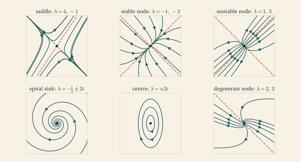
For \(n=2\) a solution \(\mathbf x(t)=(x(t),y(t))\) traces a curve in the \((x,y)\) plane, the phase plane. The curve with its direction of travel is a trajectory, and the picture of all trajectories is the phase portrait. By uniqueness, distinct trajectories do not cross. The origin is always an equilibrium of \(\mathbf x'=A\mathbf x\) , and it is the only one when \(\det A\ne0\) .

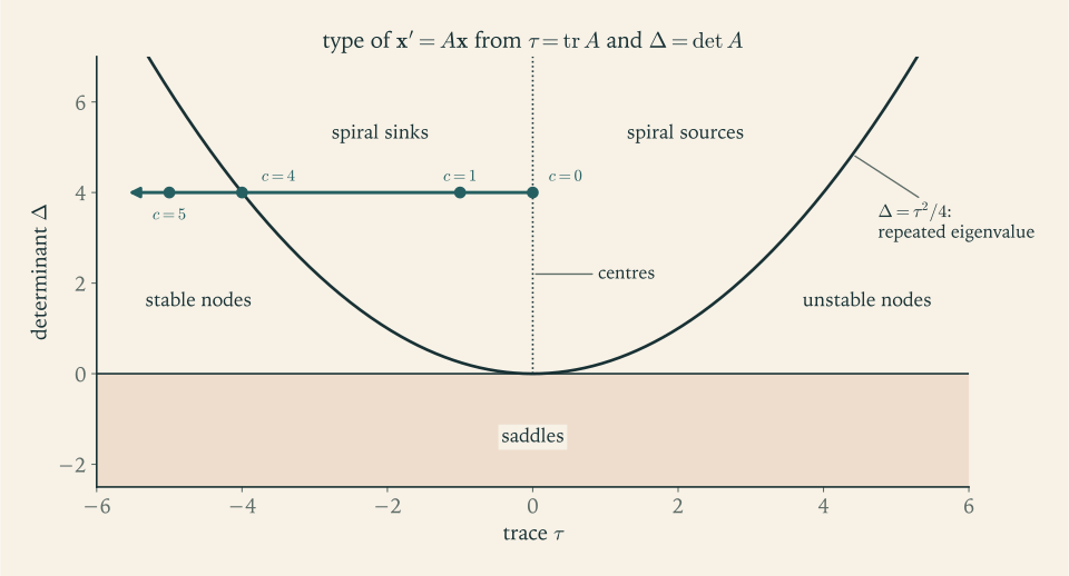
The portrait is determined by the eigenvalues, and these by two numbers: the trace \(\tau=a_{11}+a_{22}\) and the determinant \(\Delta=\det A\) . The characteristic polynomial is \(\lambda^2-\tau\lambda+\Delta\) , so

What the names mean geometrically follows from the solution formulas.

At a saddle, \(\mathbf x=c_1e^{\lambda_1t}\mathbf v_1+c_2e^{\lambda_2t}\mathbf v_2\) with \(\lambda_1>0>\lambda_2\) . Trajectories on the line through \(\mathbf v_2\) approach the origin; all others are swept away, approaching the line through \(\mathbf v_1\) .

At a stable node, both exponentials decay, and the one with the eigenvalue nearer zero decays more slowly. So every trajectory approaches the origin, and all except those on the fast eigenvector line arrive tangent to the slow eigenvector.

At a spiral, Proposition 7.4 shows rotation with period \(2\pi/\beta\) combined with growth or decay at the rate \(\tau/2\) . At a centre the trajectories are closed curves, ellipses, and every solution is periodic. The sense of rotation is found by evaluating \(A\mathbf x\) at one point: at \((1,0)\) the velocity is the first column of \(A\) , so the rotation is counterclockwise if \(a_{21}>0\) .

At a degenerate node with only one eigenvector direction, as in Example 7.5, every trajectory is tangent to that direction at the origin.

For stability the essential information is the sign of the real parts.

The statement and its proof extend to \(n\times n\) matrices, where the entries of \(e^{tA}\) involve powers of \(t\) up to \(t^{n-1}\) ; the general case uses the Jordan form from linear algebra and is quoted here without proof. The rate \(\alpha\) must in general be strictly smaller than the decay rate of the eigenvalues, because of the factor \(t\) that a repeated eigenvalue produces. And the constant \(C\) cannot always be taken to be \(1\) : Exercise 6 exhibits a stable system in which the distance of a solution from the origin grows to several times its initial value before it decays.

7.5 Forced systems

For the scalar equation \(y'=ay+g(t)\) the integrating factor \(e^{-at}\) gave \(y=e^{at}y_0+\int_0^te^{a(t-s)}g(s)\,ds\) . The matrix exponential makes the same argument work for systems.

The first term is the free response to the initial state, and the second is a convolution of the forcing with the matrix weight function \(e^{tA}\) . For the system of a second-order equation this formula contains variation of parameters (Theorem 5.3) and the convolution formula of Section 6.4.

Exercises

1. Write \(y''+5y'+6y=0\) as a system \(\mathbf x'=A\mathbf x\) for \(\mathbf x=(y,y')\) , find the eigenvalues and eigenvectors of \(A\) , and explain why every eigenvector of such a matrix has the form \((1,\lambda)\) up to a multiple.

   Answer

   \(A=\begin{pmatrix}0&1\\-6&-5\end{pmatrix}\) , with characteristic polynomial \(\lambda^2+5\lambda+6\) , eigenvalues \(-2\) and \(-3\) , and eigenvectors \((1,-2)\) and \((1,-3)\) . The first row of \((A-\lambda I)\mathbf v=\mathbf 0\) is \(-\lambda v_1+v_2=0\) , so \(v_2=\lambda v_1\) : the second component is the derivative of the first, and \(e^{\lambda t}(1,\lambda)\) is \((y,y')\) for \(y=e^{\lambda t}\) .

2. Solve \(\mathbf x'=\begin{pmatrix}4&-2\\1&1\end{pmatrix}\mathbf x\) with \(\mathbf x(0)=(1,2)\) by the eigenvalue method.

   Solution

   The characteristic polynomial is \(\det\begin{pmatrix}4-\lambda&-2\\1&1-\lambda\end{pmatrix}=\lambda^2-5\lambda+6=(\lambda-2)(\lambda-3)\) .

   For \(\lambda=2\) : \((A-2I)\mathbf v=\mathbf 0\) reads \(2v_1-2v_2=0\) , so \(\mathbf v_1=(1,1)\) . For \(\lambda=3\) : \(v_1-2v_2=0\) , so \(\mathbf v_2=(2,1)\) . The eigenvalues are distinct, so by Theorem 7.3 the general solution is

   \[ \mathbf x(t)=c_1e^{2t}\begin{pmatrix}1\\1\end{pmatrix}+c_2e^{3t}\begin{pmatrix}2\\1\end{pmatrix}. \]

   The initial vector gives \(c_1+2c_2=1\) and \(c_1+c_2=2\) . Subtracting, \(c_2=-1\) , and then \(c_1=3\) :

   \[ \mathbf x(t)=3e^{2t}\begin{pmatrix}1\\1\end{pmatrix}-e^{3t}\begin{pmatrix}2\\1\end{pmatrix}=\begin{pmatrix}3e^{2t}-2e^{3t}\\3e^{2t}-e^{3t}\end{pmatrix}. \]

   Check: \(\mathbf x(0)=(1,2)\) , and \(x_1'=6e^{2t}-6e^{3t}\) agrees with \(4x_1-2x_2=12e^{2t}-8e^{3t}-6e^{2t}+2e^{3t}\) . Both eigenvalues are positive, so the origin is an unstable node, and for large \(t\) the solution is dominated by the faster mode \(e^{3t}\) and runs off in the direction \(-(2,1)\) .

3. For \(A=\begin{pmatrix}2&-5\\1&-2\end{pmatrix}\) find the real general solution of \(\mathbf x'=A\mathbf x\) , show that \(x^2-4xy+5y^2\) is constant along every solution, and describe the trajectories.

   Solution

   Trace \(0\) and determinant \(-4+5=1\) give the characteristic polynomial \(\lambda^2+1\) , so \(\lambda=\pm i\) : a centre. For \(\lambda=i\) the first row of \(A-iI\) gives \((2-i)v_1-5v_2=0\) , satisfied by \(\mathbf v=(5,\,2-i)=(5,2)+i\,(0,-1)\) . With \(\mathbf a=(5,2)\) , \(\mathbf b=(0,-1)\) , \(\alpha=0\) , \(\beta=1\) , Proposition 7.4 gives the real general solution

   \[ \mathbf x(t)=c_1\begin{pmatrix}5\cos t\\2\cos t+\sin t\end{pmatrix}+c_2\begin{pmatrix}5\sin t\\2\sin t-\cos t\end{pmatrix}. \]

   For the conserved quantity let \(Q=x^2-4xy+5y^2\) with \(x'=2x-5y\) , \(y'=x-2y\) . Then

   \[ Q'=(2x-4y)\,x'+(-4x+10y)\,y'=(2x-4y)(2x-5y)+(-4x+10y)(x-2y). \]

   Expanding, the first product is \(4x^2-18xy+20y^2\) and the second is \(-4x^2+18xy-20y^2\) , so \(Q'=0\) .

   Since \(Q=(x-2y)^2+y^2\) is positive except at the origin, its level sets \(Q=\text{constant}\) are ellipses centred at the origin, and each trajectory stays on one of them. Every solution is periodic with period \(2\pi\) . At \((1,0)\) the velocity is \((2,1)\) , with positive second component, so the ellipses are traversed counterclockwise.

4. For \(A=\begin{pmatrix}0&-3\\3&0\end{pmatrix}\) compute \(A^2\) and use it to sum the series for \(e^{tA}\) in closed form, separating even and odd powers.

   Answer

   \(A^2=-9I\) , so \(A^{2k}=(-9)^kI\) and \(A^{2k+1}=(-9)^kA\) . The even powers sum to \(I\cos3t\) and the odd powers to \(\tfrac13A\sin3t\) : \(e^{tA}=\begin{pmatrix}\cos3t&-\sin3t\\\sin3t&\cos3t\end{pmatrix}\) , a rotation through the angle \(3t\) .

5. Compute \(e^{tA}\) for the nilpotent matrix \(A=\begin{pmatrix}0&1&2\\0&0&3\\0&0&0\end{pmatrix}\) and use it to solve \(\mathbf x'=A\mathbf x\) , \(\mathbf x(0)=(0,0,1)\) .

   Answer

   \(A^2\) has the single nonzero entry \(3\) in position \((1,3)\) and \(A^3=0\) , so \(e^{tA}=I+tA+\tfrac12t^2A^2=\begin{pmatrix}1&t&2t+\tfrac32t^2\\0&1&3t\\0&0&1\end{pmatrix}\) . The solution is the third column, \(\mathbf x(t)=(2t+\tfrac32t^2,\,3t,\,1)\) .

6. For \(A=\begin{pmatrix}-1&10\\0&-1\end{pmatrix}\) find \(e^{tA}\) and show that every solution of \(\mathbf x'=A\mathbf x\) tends to \(\mathbf 0\) . Then show that for \(\mathbf x(0)=(0,1)\) the distance \(\lVert\mathbf x(t)\rVert\) from the origin nevertheless grows before it decays, find the time and size of its maximum, and say what this implies about the constants \(C\) and \(\alpha\) in Theorem 7.8.

   Solution

   The matrix is \(A=-I+10N\) with \(N=\begin{pmatrix}0&1\\0&0\end{pmatrix}\) and \(N^2=0\) . Since \(-I\) commutes with \(N\) ,

   \[ e^{tA}=e^{-t}(I+10tN)=e^{-t}\begin{pmatrix}1&10t\\0&1\end{pmatrix}. \]

   A solution is \(\mathbf x(t)=e^{tA}\mathbf x_0=e^{-t}\bigl(x_{0,1}+10t\,x_{0,2},\ x_{0,2}\bigr)\) . Both \(e^{-t}\) and \(te^{-t}\) tend to \(0\) as \(t\to\infty\) , so every solution tends to \(\mathbf 0\) ; the repeated eigenvalue \(-1\) is negative, as Theorem 7.8 requires.

   For \(\mathbf x(0)=(0,1)\) : \(\mathbf x(t)=e^{-t}(10t,\,1)\) , so \(\lVert\mathbf x(t)\rVert^2=e^{-2t}(1+100t^2)\) and

   \[ \frac{d}{dt}\lVert\mathbf x(t)\rVert^2=e^{-2t}\bigl(200t-2-200t^2\bigr)=-2e^{-2t}\bigl(100t^2-100t+1\bigr). \]

   The quadratic has the roots \(t=\tfrac12\bigl(1\pm\sqrt{0.96}\bigr)\) , about \(0.010\) and \(0.990\) , and is negative between them. So the distance decreases very briefly, then increases until \(t\approx0.990\) , and decreases from then on. Its maximum is \(e^{-0.990}\sqrt{1+100\,(0.990)^2}\approx3.70\) : the solution starts at distance \(1\) from the origin and travels to distance \(3.70\) before it begins to return.

   In the bound \(\lVert e^{tA}\mathbf x_0\rVert\le Ce^{-\alpha t}\lVert\mathbf x_0\rVert\) this forces \(C\ge3.70\,e^{0.990\,\alpha}>3.70\) : the constant cannot be \(1\) . It also forces \(\alpha<1\) , because \(10t\,e^{-t}\) is not bounded by any multiple of \(e^{-t}\) ; any \(\alpha<1\) is possible, at the price of a larger \(C\) .

   Growth of one component is not enough for this conclusion. For \(\begin{pmatrix}-1&1\\0&-1\end{pmatrix}\) and the same start, the first component \(te^{-t}\) rises to \(e^{-1}\) , yet the distance \(e^{-t}\sqrt{1+t^2}\) decreases for all \(t>0\) , and there \(C=1\) works with \(\alpha=\tfrac12\) . Transient growth of the distance needs a sufficiently strong coupling between the variables.

7. Classify the equilibrium at the origin for each matrix using trace and determinant, and state whether it is stable: (a) \(\begin{pmatrix}2&1\\1&2\end{pmatrix}\) ; (b) \(\begin{pmatrix}-1&-4\\1&-1\end{pmatrix}\) ; (c) \(\begin{pmatrix}1&3\\1&-1\end{pmatrix}\) ; (d) \(\begin{pmatrix}0&2\\-2&0\end{pmatrix}\) ; (e) \(\begin{pmatrix}-3&0\\0&-3\end{pmatrix}\) .

   Answer

   (a) \(\tau=4\) , \(\Delta=3\) , \(\tau^2-4\Delta=4>0\) : unstable node. (b) \(\tau=-2\) , \(\Delta=5\) , \(\tau^2-4\Delta=-16\) : stable spiral, counterclockwise. (c) \(\Delta=-4\) : saddle, unstable. (d) \(\tau=0\) , \(\Delta=4\) : centre, clockwise; solutions stay bounded but do not tend to the origin. (e) \(\tau=-6\) , \(\Delta=9\) , \(\tau^2=4\Delta\) : a degenerate stable node in which every direction is an eigenvector, so trajectories are straight rays into the origin.

8. The damped oscillator \(y''+cy'+y=0\) with \(c\ge0\) corresponds to the matrix \(\begin{pmatrix}0&1\\-1&-c\end{pmatrix}\) . Classify the origin for every value of \(c\) and match each type with the terms undamped, underdamped, critically damped, and overdamped of Chapter 4.

   Answer

   \(\tau=-c\) , \(\Delta=1\) , \(\tau^2-4\Delta=c^2-4\) . For \(c=0\) a centre (undamped); for \(0<c<2\) a stable spiral (underdamped); for \(c=2\) a degenerate stable node (critically damped); for \(c>2\) a stable node (overdamped).

9. Verify by direct multiplication that every \(2\times2\) matrix \(A\) with trace \(\tau\) and determinant \(\Delta\) satisfies \(A^2-\tau A+\Delta I=0\) , and deduce that if \(A\) has a repeated eigenvalue \(\lambda\) then \((A-\lambda I)^2=0\) .

   Hint

   Write \(A=\begin{pmatrix}a&b\\c&d\end{pmatrix}\) and compute \(A^2-(a+d)A+(ad-bc)I\) entry by entry. For a repeated eigenvalue, \(\tau=2\lambda\) and \(\Delta=\lambda^2\) .

10. Prove from the series that if \(A\mathbf v=\lambda\mathbf v\) then \(e^{tA}\mathbf v=e^{\lambda t}\mathbf v\) , and use Theorem 7.6(c) to prove that two solutions of \(\mathbf x'=A\mathbf x\) that start at different points are at different points at every later time.

    Hint

    \(A^k\mathbf v=\lambda^k\mathbf v\) , so the series for \(e^{tA}\mathbf v\) is \(\bigl(\sum(\lambda t)^k/k!\bigr)\mathbf v\) . For the second part, \(e^{tA}\mathbf x_0=e^{tA}\mathbf z_0\) can be multiplied by \(e^{-tA}\) .

11. A student computes \(e^{tA}\) for \(A=\begin{pmatrix}1&2\\0&3\end{pmatrix}\) as \(\begin{pmatrix}e^{t}&e^{2t}\\1&e^{3t}\end{pmatrix}\) by exponentiating each entry of \(tA\) . Give two quick tests that this answer fails, and compute the correct matrix.

    Solution

    Two tests. At \(t=0\) the proposed matrix is \(\begin{pmatrix}1&1\\1&1\end{pmatrix}\) , but \(e^{0A}=I\) . And each column of \(e^{tA}\) must be a solution of \(\mathbf x'=A\mathbf x\) : the first column \((e^{t},1)\) has derivative \((e^{t},0)\) , while \(A(e^{t},1)=(e^{t}+2,\,3)\) . Either test rejects the answer. The entry \(1\) in the lower left is suspicious on its own, because powers of an upper triangular matrix are upper triangular and so is \(e^{tA}\) .

    The correct matrix. \(A\) is triangular with eigenvalues \(1\) and \(3\) . For \(\lambda=1\) : \(2v_2=0\) , so \(\mathbf v_1=(1,0)\) . For \(\lambda=3\) : \(-2v_1+2v_2=0\) , so \(\mathbf v_2=(1,1)\) . With

    \[ P=\begin{pmatrix}1&1\\0&1\end{pmatrix},\qquad P^{-1}=\begin{pmatrix}1&-1\\0&1\end{pmatrix}, \]

    Theorem 7.6(e) gives

    \[ e^{tA}=P\begin{pmatrix}e^{t}&0\\0&e^{3t}\end{pmatrix}P^{-1}=\begin{pmatrix}e^{t}&e^{3t}-e^{t}\\0&e^{3t}\end{pmatrix}. \]

    This equals \(I\) at \(t=0\) , and its derivative at \(t=0\) is \(\begin{pmatrix}1&2\\0&3\end{pmatrix}=A\) . The off-diagonal entry \(e^{3t}-e^{t}\) is not the exponential of anything simple; it records how the second variable drives the first.

12. Let \(A=\begin{pmatrix}0&1\\0&0\end{pmatrix}\) and \(B=\begin{pmatrix}0&0\\-1&0\end{pmatrix}\) . Compute \(e^{tA}e^{tB}\) and \(e^{t(A+B)}\) , show that they differ, and identify the hypothesis of Theorem 7.6 that is not satisfied.

    Solution

    Both matrices are nilpotent with square zero, so \(e^{tA}=I+tA\) and \(e^{tB}=I+tB\) :

    \[ e^{tA}e^{tB}=\begin{pmatrix}1&t\\0&1\end{pmatrix}\begin{pmatrix}1&0\\-t&1\end{pmatrix}=\begin{pmatrix}1-t^2&t\\-t&1\end{pmatrix}. \]

    The sum is \(J=A+B=\begin{pmatrix}0&1\\-1&0\end{pmatrix}\) , with \(J^2=-I\) . Separating even and odd powers in the series, \(e^{tJ}=I\cos t+J\sin t\) :

    \[ e^{t(A+B)}=\begin{pmatrix}\cos t&\sin t\\-\sin t&\cos t\end{pmatrix}. \]

    The two differ for every \(t\ne0\) : for instance the lower right entries are \(1\) and \(\cos t\) . They agree to first order in \(t\) , since both are \(I+t(A+B)+\dots\) , and differ at order \(t^2\) .

    Theorem 7.6(d) assumes \(AB=BA\) . Here \(AB=\begin{pmatrix}-1&0\\0&0\end{pmatrix}\) and \(BA=\begin{pmatrix}0&0\\0&-1\end{pmatrix}\) , which are different. The qualitative difference is large: \(e^{t(A+B)}\) is a rotation, bounded for all \(t\) , while the product of the two shears grows like \(t^2\) .

13. Use Theorem 7.9 to solve \(\mathbf x'=\begin{pmatrix}0&1\\-1&0\end{pmatrix}\mathbf x+\begin{pmatrix}0\\1\end{pmatrix}\) with \(\mathbf x(0)=\mathbf 0\) , and check that the first component agrees with the solution of \(y''+y=1\) from rest found in Exercise 5.18.

    Solution

    Here \(A=J\) with \(J^2=-I\) , so as in Exercise 7.12, \(e^{tA}=\begin{pmatrix}\cos t&\sin t\\-\sin t&\cos t\end{pmatrix}\) . With \(\mathbf x_0=\mathbf 0\) and \(\mathbf g=(0,1)\) , Theorem 7.9 gives

    \[ \mathbf x(t)=\int_0^te^{(t-s)A}\begin{pmatrix}0\\1\end{pmatrix}ds=\int_0^t\begin{pmatrix}\sin(t-s)\\\cos(t-s)\end{pmatrix}ds , \]

    because \(e^{(t-s)A}\) applied to \((0,1)\) is its second column. Integrating, \(\int_0^t\sin(t-s)\,ds=1-\cos t\) and \(\int_0^t\cos(t-s)\,ds=\sin t\) , so

    \[ \mathbf x(t)=\begin{pmatrix}1-\cos t\\\sin t\end{pmatrix}. \]

    The system is the first-order form of \(y''+y=1\) with \(\mathbf x=(y,y')\) : the first equation is \(y'=x_2\) and the second is \(x_2'=-y+1\) . So \(y=1-\cos t\) , which is the result of Exercise 5.18 with \(\omega_0=1\) , and the second component is its derivative. In the phase plane the trajectory is the circle of radius \(1\) about the displaced equilibrium \((1,0)\) , starting at the origin.

14. A drug moves between blood (\(x_1\) ) and tissue (\(x_2\) ) and is eliminated from the blood: \(x_1'=-3x_1+2x_2\) , \(x_2'=2x_1-2x_2\) , with time in hours. Find the eigenvalues, explain why both compartments eventually empty, and find the half-life of the slow phase of the decay.

    Answer

    \(\lambda^2+5\lambda+2=0\) , so \(\lambda=\tfrac12(-5\pm\sqrt{17})\approx-0.438\) and \(-4.562\) . Both are negative (\(\tau=-5<0\) , \(\Delta=2>0\) ), so every solution tends to \(\mathbf 0\) : the drug is eventually eliminated. After the fast mode has died, amounts decay like \(e^{-0.438t}\) , with half-life \(\ln2/0.438\approx1.58\) hours.

15. Suppose every eigenvalue of the \(2\times2\) matrix \(A\) has negative real part and \(\mathbf b\) is a constant vector. Prove that \(A\) is invertible and that every solution of \(\mathbf x'=A\mathbf x+\mathbf b\) tends to \(-A^{-1}\mathbf b\) as \(t\to\infty\) .

    Solution

    The determinant of \(A\) is the product of its eigenvalues. If both are real and negative the product is positive; if they are a complex conjugate pair the product is the square of their modulus, also positive. So \(\det A\ne0\) and \(A\) is invertible.

    Let \(\mathbf x^{*}=-A^{-1}\mathbf b\) , so that \(A\mathbf x^{*}+\mathbf b=\mathbf 0\) : this is the unique equilibrium. Given any solution \(\mathbf x\) , put \(\mathbf y(t)=\mathbf x(t)-\mathbf x^{*}\) . Then

    \[ \mathbf y'=\mathbf x'=A\mathbf x+\mathbf b=A(\mathbf y+\mathbf x^{*})+\mathbf b=A\mathbf y+(A\mathbf x^{*}+\mathbf b)=A\mathbf y . \]

    So \(\mathbf y\) solves the homogeneous system, and \(\mathbf y(t)=e^{tA}\mathbf y(0)\) . By Theorem 7.8 there are constants \(C\) and \(\alpha>0\) with \(\lVert\mathbf y(t)\rVert\le Ce^{-\alpha t}\lVert\mathbf y(0)\rVert\) , which tends to \(0\) . Hence \(\mathbf x(t)\to\mathbf x^{*}=-A^{-1}\mathbf b\) , whatever the initial value. Shifting the origin to the equilibrium turns a constant forcing into no forcing at all.

16. Verify that \(\Phi(t)=\begin{pmatrix}e^{t}&e^{-t}\\e^{t}&-e^{-t}\end{pmatrix}\) is a fundamental matrix for \(\mathbf x'=\begin{pmatrix}0&1\\1&0\end{pmatrix}\mathbf x\) , and compute \(e^{tA}=\Phi(t)\Phi(0)^{-1}\) in terms of hyperbolic functions.

    Answer

    The columns are \(e^{t}(1,1)\) and \(e^{-t}(1,-1)\) , eigen-solutions for \(\lambda=\pm1\) , and \(\det\Phi=-2\ne0\) . With \(\Phi(0)^{-1}=\tfrac12\begin{pmatrix}1&1\\1&-1\end{pmatrix}\) , \(e^{tA}=\begin{pmatrix}\cosh t&\sinh t\\\sinh t&\cosh t\end{pmatrix}\) .

17. Let \(\Phi(t)\) be a fundamental matrix of a \(2\times2\) system \(\mathbf x'=A\mathbf x\) . Show that \(w(t)=\det\Phi(t)\) satisfies \(w'=(\operatorname{tr}A)\,w\) , and explain how this contains Abel’s formula of Chapter 4 for \(y''+py'+qy=0\) with constant \(p\) , \(q\) .

    Hint

    Differentiate \(\det\Phi=\phi_{11}\phi_{22}-\phi_{12}\phi_{21}\) and substitute \(\Phi'=A\Phi\) row by row; the terms with off-diagonal entries of \(A\) cancel. For the companion matrix of \(y''+py'+qy=0\) the trace is \(-p\) and \(\det\Phi\) is the Wronskian.

18. A planar linear system has trajectories that approach the origin tangent to the line \(y=x\) , and the line \(y=-2x\) is also made up of trajectories, along which the decay is four times as fast. Construct a matrix \(A\) with these properties and verify its trace, determinant, and type.

    Solution

    Trajectories of a node approach the origin tangent to the eigenvector whose eigenvalue is nearer zero. So the slow eigenvector is \((1,1)\) , the direction of \(y=x\) , and the line \(y=-2x\) is the fast eigenvector direction \((1,-2)\) . Decay requires negative eigenvalues, and the fast one is four times the slow one. The simplest choice is \(\lambda_1=-1\) and \(\lambda_2=-4\) .

    Build \(A=PDP^{-1}\) with

    \[ P=\begin{pmatrix}1&1\\1&-2\end{pmatrix},\qquad D=\begin{pmatrix}-1&0\\0&-4\end{pmatrix},\qquad P^{-1}=\frac13\begin{pmatrix}2&1\\1&-1\end{pmatrix}. \]

    Then \(DP^{-1}=\dfrac13\begin{pmatrix}-2&-1\\-4&4\end{pmatrix}\) and

    \[ A=\frac13\begin{pmatrix}1&1\\1&-2\end{pmatrix}\begin{pmatrix}-2&-1\\-4&4\end{pmatrix}=\begin{pmatrix}-2&1\\2&-3\end{pmatrix}. \]

    Verification: \(A(1,1)=(-1,-1)\) and \(A(1,-2)=(-4,8)=-4\,(1,-2)\) . The trace is \(-5=\lambda_1+\lambda_2\) and the determinant is \(6-2=4=\lambda_1\lambda_2\) ; since \(\tau^2-4\Delta=9>0\) with \(\tau<0\) and \(\Delta>0\) , the origin is a stable node. Any matrix \(P\,\mathrm{diag}(-k,-4k)\,P^{-1}\) with \(k>0\) has the same phase portrait, traversed at a different speed.