A mass hanging on a spring, pulled down and released, bobs up and down. With suitable units its displacement obeys \(y''+y=0\) , and two solutions are known to every calculus student: \(\cos t\) and \(\sin t\) . Any combination \(c_1\cos t+c_2\sin t\) is again a solution. Are there others?
The question is sharper than it looks. One could try \(e^{it}\) , or \(\cos(t-1)\) , or a power series, and each turns out to be a combination of \(\cos t\) and \(\sin t\) in disguise. But checking candidates one at a time proves nothing about the candidates not yet thought of. What is needed is an argument that the solutions of \(y''+y=0\) form a family with exactly two free constants, no more and no fewer, and that \(\cos t\) and \(\sin t\) account for all of it. The argument exists, it works for every linear second-order equation, and it rests on a single fact proved in Chapter 3: an initial value problem for such an equation has one and only one solution. This chapter develops that structure and then the methods, characteristic roots, reduction of order, and power series, that produce the two basic solutions in practice.
4.1 Linearity and what it buys
Throughout this chapter \(I\) is an open interval and \(p\) , \(q\) , \(g\) are continuous functions on \(I\) . Write
The equation \(L[y]=0\) is the homogeneous equation and \(L[y]=g\) the nonhomogeneous one. An equation given as \(a(t)y''+b(t)y'+c(t)y=f(t)\) is brought to this form by dividing by \(a(t)\) , which requires \(a(t)\ne0\) on \(I\) ; points where \(a\) vanishes are singular points and must be excluded from \(I\) .
Theorem 4.1 (existence and uniqueness for linear equations). For every \(t_0\in I\) and all real numbers \(y_0\) , \(v_0\) , the initial value problem
has exactly one solution, and it is defined on all of \(I\) .
This is the statement obtained at the end of Section 3.7 by writing the equation as a first-order system and applying Theorem 3.11. Two initial values are needed because the state of a second-order system at one instant consists of position and velocity.
Theorem 4.2 (superposition). If \(y_1\) and \(y_2\) are twice differentiable on \(I\) and \(c_1\) , \(c_2\) are constants, then \(L[c_1y_1+c_2y_2]=c_1L[y_1]+c_2L[y_2]\) . Consequently every linear combination of solutions of \(L[y]=0\) is a solution of \(L[y]=0\) .
Proof. Differentiation is linear, so \((c_1y_1+c_2y_2)''+p\,(c_1y_1+c_2y_2)'+q\,(c_1y_1+c_2y_2)=c_1(y_1''+py_1'+qy_1)+c_2(y_2''+py_2'+qy_2)\) .
In the language of linear algebra, the solutions of the homogeneous equation form a vector space of functions. The main theorem of the chapter computes its dimension.
Common mistake. Superposing solutions of an equation that is not both linear and homogeneous. The functions \(y_1=1+e^{t}\) and \(y_2=1+e^{-t}\) both satisfy \(y''-y=-1\) , but \(L[y_1+y_2]=L[y_1]+L[y_2]=-2\) , so their sum does not. For the nonlinear equation \(y''=-y^3\) even a constant multiple of a solution generally fails to be a solution. Before adding solutions, check that the right-hand side is zero and that \(y\) , \(y'\) , \(y''\) appear only to the first power.
4.2 The Wronskian and fundamental sets
Given two solutions \(y_1\) , \(y_2\) of \(L[y]=0\) , when can every solution be written as \(c_1y_1+c_2y_2\) ? To match initial data \(y_0\) , \(v_0\) at \(t_0\) the constants must satisfy
a linear system that is solvable for every right-hand side exactly when its determinant is not zero.
Definition 4.3 (Wronskian). The Wronskian of two differentiable functions \(y_1\) , \(y_2\) is the function
Theorem 4.4 (Abel’s formula). If \(y_1\) and \(y_2\) are solutions of \(y''+p(t)y'+q(t)y=0\) on \(I\) , then their Wronskian satisfies \(W'=-p(t)\,W\) , so for any \(t_0\in I\)
In particular \(W\) is either zero at every point of \(I\) or zero at no point of \(I\) .
Proof. Differentiating, \(W'=y_1y_2''+y_1'y_2'-y_1'y_2'-y_1''y_2=y_1y_2''-y_1''y_2\) . Substitute \(y_i''=-py_i'-qy_i\) : the terms with \(q\) cancel and \(W'=-p\,(y_1y_2'-y_1'y_2)=-pW\) . This is a first-order linear equation for \(W\) , and Theorem 2.3 gives the formula. An exponential is never zero, so \(W(t)\) vanishes exactly when \(W(t_0)\) does.
Theorem 4.5 (fundamental sets of solutions). Let \(y_1\) , \(y_2\) be solutions of \(L[y]=0\) on \(I\) . The following are equivalent.
(a) \(W[y_1,y_2](t_0)\ne0\) for some \(t_0\in I\) .
(b) Every solution of \(L[y]=0\) on \(I\) can be written as \(c_1y_1+c_2y_2\) , and the constants are unique.
(c) \(y_1\) and \(y_2\) are linearly independent on \(I\) : if \(c_1y_1+c_2y_2\) is the zero function, then \(c_1=c_2=0\) .
Solutions with these properties exist. Hence the solution space of \(L[y]=0\) has dimension exactly two.
Proof. (a) implies (b). Let \(y\) be any solution. Because \(W(t_0)\ne0\) , the linear system displayed above, with \(y_0=y(t_0)\) and \(v_0=y'(t_0)\) , has a unique solution \((c_1,c_2)\) . The function \(c_1y_1+c_2y_2\) is a solution by superposition, and it has the same value and derivative at \(t_0\) as \(y\) . By the uniqueness in Theorem 4.1 the two functions are equal on \(I\) . The constants are unique because they are determined by the values at \(t_0\) .
(b) implies (c). The zero function is a solution, and it equals \(0\cdot y_1+0\cdot y_2\) . By the uniqueness of the constants in (b), no other combination gives it.
(c) implies (a). Suppose \(W(t_0)=0\) for some, hence by Abel’s formula every, \(t_0\) . Then the homogeneous linear system with coefficient matrix of determinant \(W(t_0)\) has a solution \((c_1,c_2)\ne(0,0)\) . The solution \(c_1y_1+c_2y_2\) then has value \(0\) and derivative \(0\) at \(t_0\) , as does the zero solution, so by uniqueness it is the zero function. That contradicts (c).
Existence. By Theorem 4.1 there are solutions \(y_1\) with data \((1,0)\) and \(y_2\) with data \((0,1)\) at \(t_0\) . Their Wronskian at \(t_0\) is \(1\) .
A pair of solutions with these properties is a fundamental set, and \(c_1y_1+c_2y_2\) is then the general solution. For \(y''+y=0\) the Wronskian of \(\cos t\) and \(\sin t\) is \(\cos^2t+\sin^2t=1\) , so they are a fundamental set, and the question that opened the chapter is settled: there are no other solutions.
Notice how each hypothesis was used. Uniqueness made a solution a prisoner of its data at one point; existence supplied a solution for every choice of data; linearity let the two-dimensional space of data be matched with a two-dimensional space of functions.
Example 4.1: A Wronskian that vanishes at a singular point
The equation \(t^2y''-2ty'+2y=0\) has the solutions \(y_1=t\) and \(y_2=t^2\) , as substitution shows: \(0-2t+2t=0\) and \(2t^2-4t^2+2t^2=0\) . Their Wronskian is
In normal form the equation is \(y''-\dfrac2t\,y'+\dfrac2{t^2}\,y=0\) , with \(p=-2/t\) , and Abel’s formula predicts \(W=C\exp\bigl(\int\tfrac2t\,dt\bigr)=Ct^2\) , in agreement.
The Wronskian vanishes at \(t=0\) and nowhere else. This does not contradict Theorem 4.4, because \(t=0\) is a singular point: \(p\) and \(q\) are not continuous there, and the theorems apply on \(I=(0,\infty)\) or on \(I=(-\infty,0)\) separately. On \((0,\infty)\) , \(W>0\) , so \(\{t,t^2\}\) is a fundamental set and the general solution is \(c_1t+c_2t^2\) .
To solve the initial value problem \(y(1)=3\) , \(y'(1)=4\) : the system is \(c_1+c_2=3\) , \(c_1+2c_2=4\) , so \(c_2=1\) , \(c_1=2\) , and \(y=2t+t^2\) . At the singular point the theory fails visibly: every solution \(c_1t+c_2t^2\) has \(y(0)=0\) , so the data \(y(0)=1\) cannot be met, while the data \(y(0)=0\) , \(y'(0)=1\) are met by \(t+c_2t^2\) for every \(c_2\) .
4.3 Constant coefficients
For \(ay''+by'+cy=0\) with real constants and \(a\ne0\) , the coefficients are continuous on \(\mathbb R\) , so all solutions live on \(\mathbb R\) . An exponential \(e^{rt}\) is reproduced by differentiation up to a factor, so substitute it:
Thus \(e^{rt}\) is a solution exactly when \(r\) is a root of the characteristic equation \(ar^2+br+c=0\) . This remains true for complex \(r\) , with \(e^{(\lambda+i\mu)t}=e^{\lambda t}(\cos\mu t+i\sin\mu t)\) , since the rule \((e^{rt})'=re^{rt}\) holds for complex \(r\) as well. And because the coefficients are real, the real and imaginary parts of a complex-valued solution \(u+iv\) are themselves solutions: \(L[u+iv]=L[u]+iL[v]=0\) forces \(L[u]=0\) and \(L[v]=0\) .
Theorem 4.6 (general solution for constant coefficients). Let \(r_1\) , \(r_2\) be the roots of \(ar^2+br+c=0\) , with \(a,b,c\) real and \(a\ne0\) . A fundamental set of solutions of \(ay''+by'+cy=0\) on \(\mathbb R\) is:
(a) \(e^{r_1t},\ e^{r_2t}\) if the roots are real and distinct;
(b) \(e^{rt},\ te^{rt}\) if \(r_1=r_2=r\) ;
(c) \(e^{\lambda t}\cos\mu t,\ e^{\lambda t}\sin\mu t\) if the roots are \(\lambda\pm i\mu\) with \(\mu\ne0\) .
Proof. In each case we check that both functions are solutions and that their Wronskian is not zero; Theorem 4.5 does the rest.
(a) Both are solutions by the computation above, and \(W=e^{r_1t}r_2e^{r_2t}-r_1e^{r_1t}e^{r_2t}=(r_2-r_1)e^{(r_1+r_2)t}\ne0\) .
(b) Here \(r=-b/(2a)\) , so \(2ar+b=0\) . For \(y=te^{rt}\) we have \(y'=(1+rt)e^{rt}\) and \(y''=(2r+r^2t)e^{rt}\) , hence
The Wronskian of \(e^{rt}\) and \(te^{rt}\) is \(e^{rt}(1+rt)e^{rt}-re^{rt}te^{rt}=e^{2rt}\ne0\) .
(c) The two functions are the real and imaginary parts of the complex solution \(e^{(\lambda+i\mu)t}\) , so they are solutions. A direct computation gives \(W=\mu e^{2\lambda t}\ne0\) .
The three cases correspond to three kinds of behaviour: pure exponential growth or decay; exponential behaviour modified by a factor of \(t\) ; and oscillation inside an exponential envelope. The sign of the real parts of the roots decides whether solutions decay, and the imaginary part gives the angular frequency of oscillation.
A combination \(A\cos\mu t+B\sin\mu t\) is a single sinusoid. Putting \(R=\sqrt{A^2+B^2}\) and choosing the angle \(\delta\) with \(\cos\delta=A/R\) , \(\sin\delta=B/R\) ,
\(R\) is the amplitude and \(\delta\) the phase. This amplitude-phase form shows at once the size of an oscillation and the times of its zeros and peaks.
Example 4.2: One initial value problem of each kind
Distinct real roots. \(y''-3y'+2y=0\) , \(y(0)=1\) , \(y'(0)=0\) . The characteristic equation \(r^2-3r+2=0\) has roots \(1\) and \(2\) , so \(y=c_1e^{t}+c_2e^{2t}\) . The data give \(c_1+c_2=1\) and \(c_1+2c_2=0\) , so \(c_2=-1\) , \(c_1=2\) :
Complex roots. \(y''+2y'+5y=0\) , \(y(0)=1\) , \(y'(0)=1\) . The roots of \(r^2+2r+5=0\) are \(-1\pm2i\) , so \(y=e^{-t}(A\cos2t+B\sin2t)\) . Then \(y(0)=A=1\) and \(y'(0)=-A+2B=1\) gives \(B=1\) :
The solution oscillates with angular frequency \(2\) inside the envelope \(\pm\sqrt2\,e^{-t}\) , and its first zero is where \(2t-\pi/4=\pi/2\) , at \(t=3\pi/8\approx1.178\) .
A repeated root. \(y''+2y'+y=0\) , \(y(0)=1\) , \(y'(0)=0\) . The characteristic equation is \((r+1)^2=0\) , so \(y=(c_1+c_2t)e^{-t}\) . Then \(y(0)=c_1=1\) and \(y'(0)=c_2-c_1=0\) gives \(c_2=1\) :
This solution is positive for all \(t\ge0\) and decays without oscillating.
Common mistake. Writing \(c_1e^{rt}+c_2e^{rt}\) for a repeated root. That expression is \((c_1+c_2)e^{rt}\) , a one-parameter family, and it cannot satisfy two independent initial conditions: for the last problem above it would require \(c=1\) from \(y(0)=1\) and \(-c=0\) from \(y'(0)=0\) . Whenever a proposed general solution of a second-order equation cannot match arbitrary values of \(y(t_0)\) and \(y'(t_0)\) , its two functions are dependent. The Wronskian of \(e^{rt}\) with itself is zero.
The same method handles constant-coefficient equations of any order. An equation of order \(n\) has a characteristic polynomial of degree \(n\) and a solution space of dimension \(n\) ; a real root \(r\) of multiplicity \(k\) contributes \(e^{rt},te^{rt},\dots,t^{k-1}e^{rt}\) , and a pair of complex roots contributes the corresponding sines and cosines. For instance \(y'''-y''+y'-y=0\) has characteristic polynomial \((r-1)(r^2+1)\) and general solution \(c_1e^{t}+c_2\cos t+c_3\sin t\) .
4.4 Free vibrations
A mass \(m\) on a spring of stiffness \(k\) , subject to a friction force proportional to velocity with coefficient \(c\ge0\) , obeys Newton’s law
The characteristic roots are \(r=\dfrac{-c\pm\sqrt{c^2-4mk}}{2m}\) , and everything depends on the sign of \(c^2-4mk\) .
No damping, \(c=0\) . The roots are \(\pm i\omega_0\) with \(\omega_0=\sqrt{k/m}\) , the natural frequency. Solutions are \(R\cos(\omega_0t-\delta)\) : oscillation of constant amplitude with period \(2\pi/\omega_0\) .
Underdamping, \(0<c<2\sqrt{mk}\) . The roots are \(-\dfrac{c}{2m}\pm i\omega_d\) with \(\omega_d=\sqrt{\omega_0^2-\bigl(\tfrac{c}{2m}\bigr)^2}\) . Solutions are \(Re^{-ct/(2m)}\cos(\omega_dt-\delta)\) : oscillation at the reduced frequency \(\omega_d<\omega_0\) with exponentially shrinking amplitude. Successive maxima are separated by the quasi-period \(2\pi/\omega_d\) and decrease by the constant factor \(e^{-\pi c/(m\omega_d)}\) .
Critical damping, \(c=2\sqrt{mk}\) . There is one root \(r=-c/(2m)=-\omega_0\) , and solutions are \((c_1+c_2t)e^{-\omega_0t}\) .
Overdamping, \(c>2\sqrt{mk}\) . There are two distinct negative roots, and solutions are \(c_1e^{r_1t}+c_2e^{r_2t}\) .
Proposition 4.7 (no oscillation at or above critical damping). If \(c\ge2\sqrt{mk}\) , a solution of \(my''+cy'+ky=0\) that is not identically zero vanishes for at most one value of \(t\) .
Proof. In the overdamped case \(y=e^{r_1t}\bigl(c_1+c_2e^{(r_2-r_1)t}\bigr)\) with \(r_1\ne r_2\) . If \(c_2=0\) then \(c_1\ne0\) and \(y\) never vanishes. Otherwise \(y(t)=0\) requires \(e^{(r_2-r_1)t}=-c_1/c_2\) , and a strictly monotone exponential takes each value at most once. In the critical case \(y=(c_1+c_2t)e^{rt}\) vanishes only where the polynomial \(c_1+c_2t\) does, which is at most one point unless \(c_1=c_2=0\) .
The physical bookkeeping is done by the energy \(E=\tfrac12m(y')^2+\tfrac12ky^2\) , kinetic plus potential. Along any solution,
Without damping energy is conserved; with damping it is dissipated at the rate \(c\,(y')^2\) , whatever the regime.
Example 4.3: Three dampers on one spring
Take \(m=1\) , \(k=4\) , so \(\omega_0=2\) and critical damping is \(c=2\sqrt{mk}=4\) . Release the mass from rest at \(y=1\) : \(y(0)=1\) , \(y'(0)=0\) .
With \(c=1\) the roots are \(-\tfrac12\pm i\omega_d\) , \(\omega_d=\tfrac12\sqrt{15}\approx1.936\) , and fitting the data gives
The quasi-period is \(2\pi/\omega_d\approx3.245\) , and each maximum is \(e^{-3.245/2}\approx0.197\) times the one before.
With \(c=4\) the repeated root is \(-2\) and \(y=(1+2t)e^{-2t}\) .
With \(c=5\) the roots of \(r^2+5r+4=0\) are \(-1\) and \(-4\) , and \(y=\tfrac13\bigl(4e^{-t}-e^{-4t}\bigr)\) .
At \(t=3\) the three displacements are: \(y\approx0.172\) for \(c=1\) , still oscillating inside an envelope \(\sqrt{16/15}\,e^{-t/2}\) of height about \(0.230\) ; \(7e^{-6}\approx0.017\) for \(c=4\) ; and \(\tfrac13(4e^{-3}-e^{-12})\approx0.066\) for \(c=5\) . The critically damped system is closest to rest, by a wide margin.
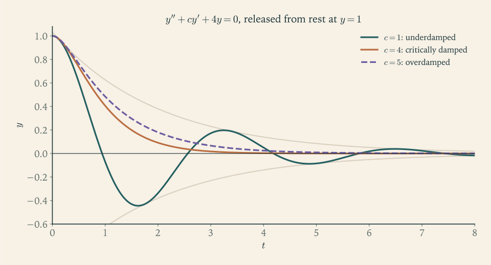
The figure makes a point that the formulas hide. Increasing \(c\) beyond the critical value slows the return, because the root nearer zero, here \(-1\) against \(-2\) , controls the long-run decay, and that root moves toward zero as \(c\) grows. Door closers and instrument needles are tuned near critical damping for this reason.
4.5 Reduction of order and Euler equations
When the coefficients are not constant there is no characteristic equation. But if one solution is known, by inspection or otherwise, the second can be computed.
Theorem 4.8 (reduction of order). Let \(y_1\) be a solution of \(y''+p(t)y'+q(t)y=0\) on \(I\) with \(y_1(t)\ne0\) for all \(t\in I\) . Then
is a solution on \(I\) , and \(\{y_1,y_2\}\) is a fundamental set.
Proof. Seek a solution of the form \(y=v\,y_1\) with \(v\) to be found. Then \(y'=v'y_1+vy_1'\) and \(y''=v''y_1+2v'y_1'+vy_1''\) , so
because \(L[y_1]=0\) . The term in \(v\) has disappeared, which leaves a first-order linear equation for \(w=v'\) : \(w'+\bigl(2y_1'/y_1+p\bigr)w=0\) . Its integrating factor is \(y_1^2e^{\int p}\) , so \(w=Ce^{-\int p}/y_1^2\) . Taking \(C=1\) and integrating once more gives \(v\) , and \(y_2=vy_1\) . Finally \(W[y_1,y_2]=y_1(v'y_1+vy_1')-y_1'vy_1=y_1^2v'=e^{-\int p}\ne0\) .
The Wronskian computed at the end is Abel’s formula again: reduction of order amounts to solving \(W[y_1,y_2]=e^{-\int p}\) for \(y_2\) .
Example 4.4: Finding the missing solution
For \(t^2y''-3ty'+4y=0\) on \((0,\infty)\) , trying a power \(y=t^r\) gives \(r(r-1)-3r+4=(r-2)^2=0\) , which produces only one solution, \(y_1=t^2\) .
In normal form \(p=-3/t\) , so \(e^{-\int p}=e^{3\ln t}=t^3\) , and
Check: \(y_2'=2t\ln t+t\) , \(y_2''=2\ln t+3\) , and \(t^2(2\ln t+3)-3t(2t\ln t+t)+4t^2\ln t=0\) . The general solution is \(y=t^2(c_1+c_2\ln t)\) .
The equation in the example is an Euler equation, \(t^2y''+\alpha ty'+\beta y=0\) with constants \(\alpha\) , \(\beta\) . Each term has the form of a power of \(t\) times a derivative of matching order, so \(t^r\) is reproduced by the left side up to a factor: substituting gives the indicial equation
For \(t>0\) , distinct real roots give \(t^{r_1}\) , \(t^{r_2}\) ; a double root gives \(t^{r}\) , \(t^{r}\ln t\) ; complex roots \(\lambda\pm i\mu\) give \(t^{\lambda}\cos(\mu\ln t)\) , \(t^{\lambda}\sin(\mu\ln t)\) . The pattern mirrors Theorem 4.6 with \(\ln t\) in place of \(t\) , and for good reason: the change of variable \(t=e^{x}\) converts an Euler equation into one with constant coefficients.
4.6 Power series solutions
Most linear equations with variable coefficients have no solution in elementary closed form, and no solution is available to start a reduction of order. A systematic method remains: look for the solution as a power series.
A function is analytic at \(t_0\) if it equals a convergent power series \(\sum_{n\ge0}c_n(t-t_0)^n\) on some interval \(\lvert t-t_0\rvert<\rho\) . A point \(t_0\) is an ordinary point of \(y''+p(t)y'+q(t)y=0\) if \(p\) and \(q\) are analytic at \(t_0\) . The method uses one fact about power series from analysis, taught in Real Analysis: inside its interval of convergence a power series may be differentiated term by term, the differentiated series has the same radius of convergence, and two power series that agree on an interval have the same coefficients.
Theorem 4.9 (series solutions at an ordinary point). Suppose \(p\) and \(q\) are given by power series in \(t-t_0\) that converge for \(\lvert t-t_0\rvert<\rho\) . Then every solution of \(y''+p(t)y'+q(t)y=0\) is given on that interval by a power series
that converges at least for \(\lvert t-t_0\rvert<\rho\) . The coefficients \(a_0=y(t_0)\) and \(a_1=y'(t_0)\) are arbitrary, and all others are determined by them through a recurrence relation.
The formal part of the theorem, that substituting a series determines \(a_2,a_3,\dots\) from \(a_0,a_1\) , is exactly the computation one carries out in each example. The substantial part is convergence with radius at least \(\rho\) ; its proof compares the recurrence with that of an equation whose series can be summed, and it is not given here. When \(p\) and \(q\) are rational functions, \(\rho\) is the distance from \(t_0\) to the nearest point of the complex plane at which a denominator vanishes.
Example 4.5: Airy’s equation
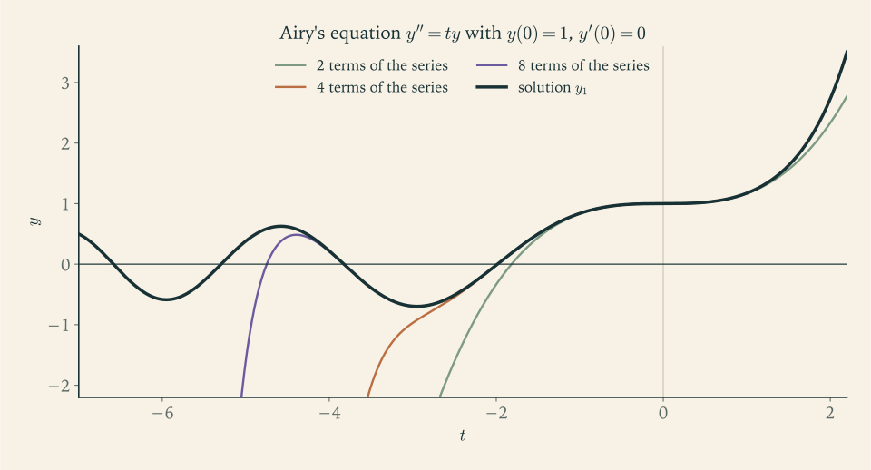
The equation \(y''-ty=0\) arises in optics and in quantum mechanics. Its coefficient \(q=-t\) is a polynomial, so every point is ordinary and series solutions about \(t_0=0\) converge for all \(t\) .
Substitute \(y=\sum_{n\ge0}a_nt^n\) . Then \(y''=\sum_{n\ge2}n(n-1)a_nt^{n-2}=\sum_{n\ge0}(n+2)(n+1)a_{n+2}t^{n}\) and \(ty=\sum_{n\ge0}a_nt^{n+1}=\sum_{n\ge1}a_{n-1}t^{n}\) . The equation becomes
Every coefficient must vanish, so \(a_2=0\) and
The recurrence links coefficients three apart. From \(a_0\) : \(a_3=a_0/6\) , \(a_6=a_3/30=a_0/180\) , \(a_9=a_6/72=a_0/12960\) . From \(a_1\) : \(a_4=a_1/12\) , \(a_7=a_4/42=a_1/504\) , \(a_{10}=a_7/90=a_1/45360\) . From \(a_2=0\) : \(a_5=a_8=\dots=0\) . Hence \(y=a_0y_1+a_1y_2\) with
These satisfy \(y_1(0)=1\) , \(y_1'(0)=0\) and \(y_2(0)=0\) , \(y_2'(0)=1\) , so their Wronskian at \(0\) is \(1\) and they form a fundamental set. Four terms give \(y_1(1)\approx1.17230\) , which agrees with a numerical integration of the initial value problem to five decimal places.
The equation itself explains the shape of the solutions better than the series does. For \(t>0\) it reads \(y''=ty\) , like \(y''=\omega^2y\) with growing \(\omega\) : solutions behave like exponentials, growing ever faster. For \(t<0\) it reads \(y''=-\lvert t\rvert y\) , like \(y''=-\omega^2y\) with \(\omega=\sqrt{\lvert t\rvert}\) : solutions oscillate, faster and faster as \(t\to-\infty\) .
Example 4.6: A radius of convergence set by complex singularities
Consider \((1+t^2)y''+2ty'=0\) about \(t_0=0\) . In normal form \(p=2t/(1+t^2)\) , which is analytic at \(0\) ; the denominator vanishes at \(t=\pm i\) , at distance \(1\) from the origin, so Theorem 4.9 guarantees convergence for \(\lvert t\rvert<1\) .
Substituting \(y=\sum a_nt^n\) and collecting the coefficient of \(t^n\) :
With \(n=0\) this gives \(a_2=0\) , hence all even coefficients beyond \(a_0\) vanish. For odd indices, \(a_3=-\tfrac13a_1\) , \(a_5=-\tfrac35a_3=\tfrac15a_1\) , \(a_7=-\tfrac57a_5=-\tfrac17a_1\) . So
The closed form can be confirmed directly: the equation is \(\bigl((1+t^2)y'\bigr)'=0\) , so \(y'=a_1/(1+t^2)\) . The series for \(\arctan t\) has radius of convergence exactly \(1\) , although \(\arctan t\) is a smooth solution on all of \(\mathbb R\) and the equation has no real singular point. The series cannot converge beyond \(\lvert t\rvert=1\) because of the singularities at \(\pm i\) , which are invisible on the real line. To continue the solution past \(t=1\) by series, one re-expands about a new centre.
At a singular point, such as \(t=0\) for an Euler equation, solutions need not be analytic, as \(t^{1/2}\) and \(t^2\ln t\) show. An extension of the series method due to Frobenius handles the commonest singular points by allowing a factor \(t^{r}\) in front of the series; it is not developed in this book.
With the homogeneous equation understood, the next chapter adds a forcing term \(g(t)\) and asks how a system responds to being driven.
Exercises
-
Solve \(y''+y'-6y=0\) with \(y(0)=1\) , \(y'(0)=2\) . Then determine, for the same equation, all pairs of initial values \(y(0)\) , \(y'(0)\) whose solutions tend to \(0\) as \(t\to\infty\) .
Answer
Roots \(2\) and \(-3\) ; \(c_1+c_2=1\) , \(2c_1-3c_2=2\) give \(c_1=1\) , \(c_2=0\) , so \(y=e^{2t}\) . A solution \(c_1e^{2t}+c_2e^{-3t}\) tends to \(0\) exactly when \(c_1=0\) , that is, when \(y'(0)=-3y(0)\) : a single line in the plane of initial data.
-
Solve \(y''+4y'+13y=0\) , \(y(0)=2\) , \(y'(0)=-1\) , write the answer in amplitude-phase form, and find the first positive time at which \(y=0\) .
Solution
The characteristic equation \(r^2+4r+13=0\) has roots \(r=-2\pm3i\) , so \(y=e^{-2t}(A\cos3t+B\sin3t)\) . From \(y(0)=2\) , \(A=2\) . Differentiating, \(y'(0)=-2A+3B=-1\) , so \(B=1\) :
\[ y=e^{-2t}(2\cos3t+\sin3t). \]For the amplitude-phase form, \(R=\sqrt{2^2+1^2}=\sqrt5\) , and \(\delta\) satisfies \(\cos\delta=2/\sqrt5\) , \(\sin\delta=1/\sqrt5\) , so \(\delta=\arctan\tfrac12\approx0.4636\) . Hence
\[ y=\sqrt5\,e^{-2t}\cos(3t-\delta). \]The exponential factor is never zero, so \(y=0\) exactly when \(\cos(3t-\delta)=0\) . Starting from \(t=0\) , where \(3t-\delta=-\delta\) lies in \((-\pi/2,0)\) , the argument increases and first reaches \(\pi/2\) when
\[ t=\frac{\pi/2+\delta}{3}\approx0.678 . \]Subsequent zeros follow at intervals of \(\pi/3\) , half the quasi-period \(2\pi/3\) .
-
Solve \(y''-6y'+9y=0\) , \(y(0)=1\) , \(y'(0)=5\) , and verify directly that your two basic solutions have a nonvanishing Wronskian.
Answer
Double root \(r=3\) : \(y=(c_1+c_2t)e^{3t}\) with \(c_1=1\) and \(3c_1+c_2=5\) , so \(y=(1+2t)e^{3t}\) . The Wronskian of \(e^{3t}\) and \(te^{3t}\) is \(e^{6t}\) , never zero.
-
Compute the Wronskian of \(e^{-t}\cos2t\) and \(e^{-t}\sin2t\) and confirm that it satisfies Abel’s formula for the equation \(y''+2y'+5y=0\) .
Answer
\(W=2e^{-2t}\) . Abel’s formula with \(p=2\) gives \(W(t)=W(0)e^{-2t}\) , and \(W(0)=1\cdot2-(-1)\cdot0=2\) .
-
Let \(y_1\) and \(y_2\) be solutions of \(y''+p(t)y'+q(t)y=0\) on \(I\) . Prove that if they vanish at the same point of \(I\) , or if they both have a local extremum at the same point of \(I\) , then they are linearly dependent.
Hint
In both cases compute the Wronskian at the common point and apply Theorem 4.5. A local extremum of a differentiable function is a zero of its derivative.
-
For Legendre’s equation \((1-t^2)y''-2ty'+2y=0\) on \((-1,1)\) , use Abel’s formula to find the Wronskian of any two solutions up to a constant, check that \(y_1=t\) is a solution, and find a second solution by reduction of order on \((0,1)\) .
Solution
In normal form the equation is \(y''-\dfrac{2t}{1-t^2}\,y'+\dfrac{2}{1-t^2}\,y=0\) , so \(p=-2t/(1-t^2)\) and \(\int p\,dt=\ln(1-t^2)\) on \((-1,1)\) . Abel’s formula gives
\[ W=C\exp\bigl(-\ln(1-t^2)\bigr)=\frac{C}{1-t^2}. \]For \(y_1=t\) : \(y_1''=0\) , and \(-2t\cdot1+2t=0\) , so it is a solution. It vanishes at \(t=0\) , so apply reduction of order on \((0,1)\) , where \(y_1\ne0\) :
\[ y_2=t\int\frac{dt}{t^2(1-t^2)} . \]By partial fractions \(\dfrac{1}{t^2(1-t^2)}=\dfrac1{t^2}+\dfrac{1}{1-t^2}\) , and \(\displaystyle\int\frac{dt}{1-t^2}=\frac12\ln\frac{1+t}{1-t}\) . Therefore
\[ y_2=t\Bigl(-\frac1t+\frac12\ln\frac{1+t}{1-t}\Bigr)=\frac t2\ln\frac{1+t}{1-t}-1 . \]Although the construction used \(t\ne0\) , the resulting formula is defined and smooth on all of \((-1,1)\) and is a solution there, with \(y_2(0)=-1\) . Its Wronskian with \(y_1\) is \(1/(1-t^2)\) , in agreement with Abel’s formula with \(C=1\) . The solution \(y_2\) is unbounded as \(t\to\pm1\) , the singular points of the equation, while \(y_1=t\) stays bounded: only a one-dimensional family of solutions is bounded on the whole interval.
-
Given that \(y_1=e^{t}\) solves \(ty''-(t+1)y'+y=0\) for \(t>0\) , find a second solution by reduction of order, simplify it to a polynomial, and verify it by substitution.
Solution
Divide by \(t\) : \(y''-\Bigl(1+\dfrac1t\Bigr)y'+\dfrac1t\,y=0\) , so \(p=-1-1/t\) and \(-\int p\,dt=t+\ln t\) , giving \(e^{-\int p}=te^{t}\) . With \(y_1=e^{t}\) , Theorem 4.8 gives
\[ v'=\frac{te^{t}}{e^{2t}}=te^{-t},\qquad v=-(t+1)e^{-t},\qquad y_2=vy_1=-(t+1). \]A constant multiple of a solution is a solution, so we may take \(y_2=t+1\) . Check: \(y_2'=1\) , \(y_2''=0\) , and
\[ t\cdot0-(t+1)\cdot1+(t+1)=0 . \]The Wronskian of \(e^{t}\) and \(t+1\) is \(e^{t}\cdot1-e^{t}(t+1)=-te^{t}\) , nonzero for \(t>0\) , so \(\{e^{t},t+1\}\) is a fundamental set on \((0,\infty)\) and the general solution is \(c_1e^{t}+c_2(t+1)\) . The Wronskian vanishes at the singular point \(t=0\) , as in Example 4.1.
-
Solve the Euler equation \(t^2y''+ty'+4y=0\) for \(t>0\) with \(y(1)=1\) , \(y'(1)=2\) , and explain why the solution has infinitely many zeros in the interval \((0,1)\) .
Answer
The indicial equation is \(r^2+4=0\) , so \(y=A\cos(2\ln t)+B\sin(2\ln t)\) . From \(y(1)=A=1\) and \(y'(1)=2B=2\) : \(y=\cos(2\ln t)+\sin(2\ln t)\) . As \(t\to0^{+}\) , \(2\ln t\) decreases through all negative numbers, so the sinusoid passes through infinitely many zeros.
-
A mass of \(2\ \mathrm{kg}\) hangs on a spring of stiffness \(50\ \mathrm{N/m}\) . Find the damping coefficient that gives critical damping, and for \(c=4\ \mathrm{N\,s/m}\) find the quasi-period and the ratio of successive maximum displacements.
Answer
Critical damping: \(c=2\sqrt{mk}=20\ \mathrm{N\,s/m}\) . For \(c=4\) : \(\omega_0=5\) , \(c/(2m)=1\) , \(\omega_d=\sqrt{24}\approx4.90\ \mathrm{rad/s}\) , quasi-period \(2\pi/\omega_d\approx1.28\ \mathrm{s}\) , and successive maxima in the ratio \(e^{-1.28}\approx0.277\) .
-
A student notes that \(y_1=t^2\) and \(y_2=t\lvert t\rvert\) have Wronskian identically zero on \(\mathbb R\) and concludes that they are linearly dependent on \(\mathbb R\) . Show that the conclusion is false and explain why Theorem 4.5 is not contradicted.
Solution
The Wronskian. For \(t\ge0\) , \(y_2=t^2=y_1\) . For \(t<0\) , \(y_2=-t^2=-y_1\) . Also \(y_2'=2\lvert t\rvert\) exists everywhere. On each half-line \(y_2\) is a constant multiple of \(y_1\) , so \(W=y_1y_2'-y_1'y_2=0\) there, and at \(t=0\) all four values are \(0\) . So \(W\) is identically zero.
Independence. Suppose \(c_1t^2+c_2t\lvert t\rvert=0\) for all real \(t\) . At \(t=1\) this gives \(c_1+c_2=0\) and at \(t=-1\) it gives \(c_1-c_2=0\) , so \(c_1=c_2=0\) . The functions are linearly independent on \(\mathbb R\) .
No contradiction. Theorem 4.5 concerns two solutions of one equation \(y''+py'+qy=0\) with \(p\) , \(q\) continuous on \(I\) . The function \(t\lvert t\rvert\) has derivative \(2\lvert t\rvert\) , which is not differentiable at \(0\) , so it is not twice differentiable on any interval containing \(0\) and cannot be a solution of a second-order equation there. On \((0,\infty)\) or on \((-\infty,0)\) separately the two functions are dependent, which is consistent with the theorem. A vanishing Wronskian proves dependence only for solutions of a common linear equation.
-
The functions \(y_1=1+e^{t}\) and \(y_2=1+e^{-t}\) satisfy \(y''-y=-1\) . A student claims that \(c_1y_1+c_2y_2\) is the general solution. Compute \(L[c_1y_1+c_2y_2]\) , determine exactly which combinations are solutions, and write the correct general solution.
Solution
With \(L[y]=y''-y\) , linearity gives
\[ L[c_1y_1+c_2y_2]=c_1L[y_1]+c_2L[y_2]=-(c_1+c_2). \]This equals the required right-hand side \(-1\) exactly when \(c_1+c_2=1\) . So of all combinations, only those with \(c_1+c_2=1\) are solutions, and they are
\[ c_1(1+e^{t})+(1-c_1)(1+e^{-t})=1+c_1e^{t}+(1-c_1)e^{-t}, \]a one-parameter family. It cannot be the general solution, which must match two arbitrary initial values.
The correct structure is one particular solution plus the general solution of the homogeneous equation \(y''-y=0\) . The constant \(1\) is a particular solution, and \(e^{t}\) , \(e^{-t}\) form a fundamental set for the homogeneous equation, so
\[ y=1+ae^{t}+be^{-t} \]with \(a\) , \(b\) arbitrary. The solutions of a nonhomogeneous equation do not form a vector space; they form a translate of one.
-
Let \(q\) be continuous with \(q(t)<0\) on an interval \(I\) . Prove that a solution of \(y''+q(t)y=0\) that is not identically zero has at most one zero in \(I\) , and say what this implies for solutions of Airy’s equation on \((0,\infty)\) .
Solution
Suppose a nonzero solution \(y\) had two zeros in \(I\) . The zeros of a nonzero solution are isolated: at a zero \(t_1\) we must have \(y'(t_1)\ne0\) , since otherwise \(y\) would have zero data at \(t_1\) and be identically zero by Theorem 4.1. So we may take two consecutive zeros \(t_1<t_2\) , with \(y\ne0\) on \((t_1,t_2)\) . Replacing \(y\) by \(-y\) if necessary, \(y>0\) on \((t_1,t_2)\) .
On that interval \(y''=-q(t)y>0\) , because \(-q>0\) and \(y>0\) . So \(y'\) is strictly increasing on \([t_1,t_2]\) . By Rolle’s theorem there is a point \(\tau\in(t_1,t_2)\) with \(y'(\tau)=0\) ; then \(y'<0\) on \((t_1,\tau)\) , so \(y\) decreases from \(y(t_1)=0\) and is negative just after \(t_1\) . That contradicts \(y>0\) on \((t_1,t_2)\) .
For Airy’s equation \(y''-ty=0\) we have \(q(t)=-t<0\) on \((0,\infty)\) , so every nonzero solution has at most one positive zero: solutions do not oscillate for \(t>0\) , in agreement with Figure 4.2.
-
Find the recurrence relation for power series solutions of \(y''+ty'+y=0\) about \(t_0=0\) , write the first four nonzero terms of the solutions \(y_1\) and \(y_2\) with \(y_1(0)=1\) , \(y_1'(0)=0\) and \(y_2(0)=0\) , \(y_2'(0)=1\) , and identify \(y_1\) in closed form.
Solution
Substitute \(y=\sum_{n\ge0}a_nt^n\) . Then \(y''=\sum_{n\ge0}(n+2)(n+1)a_{n+2}t^n\) and \(ty'=\sum_{n\ge0}na_nt^n\) , so the coefficient of \(t^n\) in \(y''+ty'+y\) is
\[ (n+2)(n+1)a_{n+2}+(n+1)a_n=0,\qquad a_{n+2}=-\frac{a_n}{n+2}. \]With \(a_0=1\) , \(a_1=0\) : \(a_2=-\tfrac12\) , \(a_4=-\tfrac14a_2=\tfrac18\) , \(a_6=-\tfrac16a_4=-\tfrac1{48}\) , so
\[ y_1=1-\frac{t^2}{2}+\frac{t^4}{8}-\frac{t^6}{48}+\cdots \]With \(a_0=0\) , \(a_1=1\) : \(a_3=-\tfrac13\) , \(a_5=-\tfrac15a_3=\tfrac1{15}\) , \(a_7=-\tfrac17a_5=-\tfrac1{105}\) , so
\[ y_2=t-\frac{t^3}{3}+\frac{t^5}{15}-\frac{t^7}{105}+\cdots \]For \(y_1\) the general even coefficient is \(a_{2k}=(-1)^k/(2\cdot4\cdots2k)=(-1)^k/(2^kk!)\) , which is the coefficient of \(t^{2k}\) in \(e^{-t^2/2}\) . So \(y_1=e^{-t^2/2}\) , and indeed \(y_1'=-te^{-t^2/2}\) , \(y_1''=(t^2-1)e^{-t^2/2}\) give \(y_1''+ty_1'+y_1=0\) . The coefficients are polynomials, so both series converge for all \(t\) .
-
Show that the equation \(y''-2ty'+4y=0\) has a polynomial solution by computing the series solution with \(a_0=1\) , \(a_1=0\) , and explain from the recurrence why the series terminates.
Answer
The recurrence is \(a_{n+2}=\dfrac{2n-4}{(n+2)(n+1)}a_n\) . With \(a_0=1\) : \(a_2=-2\) , and \(a_4=0\) because the factor \(2n-4\) vanishes at \(n=2\) ; all later even coefficients are then zero. So \(y=1-2t^2\) .
-
Without solving, use Theorem 4.9 to give a lower bound for the radius of convergence of power series solutions of \((4+t^2)y''+y=0\) about \(t_0=0\) and about \(t_0=1\) .
Answer
The denominator \(4+t^2\) vanishes at \(t=\pm2i\) . The distance from \(0\) is \(2\) , and from \(1\) it is \(\sqrt{1+4}=\sqrt5\approx2.24\) . The series converge at least for \(\lvert t\rvert<2\) and \(\lvert t-1\rvert<\sqrt5\) .
-
Find the general solution of \(y''''-y=0\) , state the dimension of its solution space, and identify the solutions that remain bounded as \(t\to\infty\) and as \(t\to-\infty\) .
Hint
Factor \(r^4-1=(r-1)(r+1)(r^2+1)\) . Which of the four basic solutions is bounded in which direction?
-
Let \(y\) be a solution of \(y''+p(t)y'+q(t)y=0\) that does not vanish on \(I\) . Show that \(u=y'/y\) satisfies the first-order Riccati equation \(u'=-u^2-p(t)u-q(t)\) , and use this with \(y''-y=0\) to solve \(u'=1-u^2\) , \(u(0)=0\) .
Solution
Since \(y\ne0\) on \(I\) , \(u=y'/y\) is differentiable, and by the quotient rule
\[ u'=\frac{y''y-(y')^2}{y^2}=\frac{y''}{y}-u^2 . \]From the equation, \(y''=-py'-qy\) , so \(y''/y=-pu-q\) , and therefore \(u'=-u^2-p(t)u-q(t)\) . So every nonvanishing solution of the linear second-order equation produces a solution of a Riccati equation, and a Riccati equation of this form can be solved by solving a linear one.
For \(y''-y=0\) we have \(p=0\) , \(q=-1\) , and the Riccati equation is \(u'=1-u^2\) . The condition \(u(0)=0\) means \(y'(0)=0\) . The solution of \(y''-y=0\) with \(y(0)=1\) , \(y'(0)=0\) is \(y=\cosh t\) , which never vanishes, so
\[ u=\frac{\sinh t}{\cosh t}=\tanh t . \]Check: \(u'=1/\cosh^2t=1-\tanh^2t\) and \(u(0)=0\) . The solution exists for all \(t\) and tends to the equilibria \(\pm1\) of \(u'=1-u^2\) as \(t\to\pm\infty\) , as the phase line predicts.
-
A lightly damped oscillator is observed to have successive maximum displacements \(1.00\) and \(0.37\) , two seconds apart. Assuming the model \(y''+2ay'+(a^2+\omega^2)y=0\) , find \(a\) and \(\omega\) and write the equation with numerical coefficients.
Answer
The roots are \(-a\pm i\omega\) . The maxima are one quasi-period apart, so \(2\pi/\omega=2\) and \(\omega=\pi\) . Their ratio is \(e^{-2a}=0.37\) , so \(a=-\tfrac12\ln0.37\approx0.497\) . The equation is \(y''+0.994\,y'+10.12\,y=0\) .