You find a bucket with a hole in its bottom, and the bucket is empty. When was it last full?
The question has no answer, and the reason is mathematical, not practical. Exercise 2.15 gave the law for the depth of water, \(h'=-k\sqrt h\) . An empty bucket satisfies it: \(h=0\) is an equilibrium. But so does a bucket that drained from any depth and reached empty one minute ago, or one hour ago. All these histories arrive at the same present state. Run time backward from “empty now” and the differential equation does not determine what happened. For an initial value problem to be a prediction, it must have a solution, and only one. The bucket shows that this is not automatic.
There is a second way for prediction to fail, already met in Example 1.1: the solution of \(y'=y^2\) , \(y(0)=1\) exists and is unique, and it ceases to exist at \(t=1\) . This chapter finds the hypothesis on \(f\) that excludes the first failure, proves that under it every initial value problem \(y'=f(t,y)\) , \(y(t_0)=y_0\) has exactly one solution near \(t_0\) , measures how far that solution depends on the initial value, and describes precisely how a solution can come to an end.
3.1 Two ways to fail
Example 3.1: Infinitely many solutions through one point
Consider \(y'=3y^{2/3}\) , \(y(0)=0\) , where \(y^{2/3}\) means \((\sqrt[3]{y})^{2}\) , a continuous nonnegative function of \(y\in\mathbb R\) .
The constant function \(y=0\) is a solution. So is \(y=t^3\) , since then \(y'=3t^2\) and \(3y^{2/3}=3(t^3)^{2/3}=3t^2\) . More generally, pick any number \(b\ge 0\) and define
For \(t<b\) both sides of the equation are \(0\) . For \(t>b\) , \(y_b'=3(t-b)^2=3y_b^{2/3}\) . At \(t=b\) the left derivative is \(0\) and the right derivative is \(\lim_{s\to0^{+}}s^3/s=0\) , so \(y_b\) is differentiable there with \(y_b'(b)=0=3y_b(b)^{2/3}\) . Hence each \(y_b\) is a solution on \(\mathbb R\) with \(y_b(0)=0\) .
The initial value problem has infinitely many solutions: the solution may sit at zero for any length of time \(b\) and then leave. The same construction on the left, with \((t-a)^3\) for \(t<a\le 0\) , gives still more. The right-hand side is a continuous function; continuity alone does not give uniqueness.
Example 3.2: A unique solution that ends
Consider \(y'=y^2\) , \(y(0)=y_0\) with \(y_0>0\) . By separation of variables (Theorem 2.2 with \(h(y)=y^2\) on \(J=(0,\infty)\) ),
The solution tends to \(+\infty\) as \(t\to1/y_0\) . The larger the initial value, the sooner the end: for \(y_0=1/2,1,2\) the solution lives until \(t=2,1,1/2\) .
The right-hand side \(y^2\) is a polynomial. No amount of smoothness of \(f\) prevents this; what matters is how fast \(f\) grows.

Compare both examples with the linear case. By Theorem 2.3 a linear equation with continuous coefficients on \(I\) has exactly one solution through each point, defined on all of \(I\) . Neither failure can occur. The task now is to find what, short of linearity, guarantees as much as possible of that.
3.2 The Lipschitz condition
What goes wrong in Example 3.1 is visible in the graph of \(3y^{2/3}\) : at \(y=0\) it has a vertical tangent. A solution sitting at \(0\) and a solution just above \(0\) are being driven apart at a rate that is not controlled by their distance. The condition that restores control is a bound on difference quotients.
Definition 3.1 (Lipschitz condition). A function \(f\) defined on a set \(D\) in the \((t,y)\) plane is Lipschitz in \(y\) on \(D\) with constant \(L\ge0\) if
for all pairs of points \((t,y_1)\) and \((t,y_2)\) in \(D\) . It is locally Lipschitz in \(y\) on an open set \(D\) if every point of \(D\) is the centre of a closed rectangle contained in \(D\) on which \(f\) is Lipschitz in \(y\) .
The condition compares two values of \(y\) at the same \(t\) , and it says the right-hand sides can differ by at most a fixed multiple of the difference in \(y\) . It is usually verified with a derivative.
Lemma 3.2 (a bounded derivative gives a Lipschitz constant). Let \(R\) be a rectangle and suppose \(\partial f/\partial y\) exists on \(R\) with \(\lvert\partial f/\partial y\rvert\le L\) there. Then \(f\) is Lipschitz in \(y\) on \(R\) with constant \(L\) . In particular, if \(f\) and \(\partial f/\partial y\) are continuous on an open set \(D\) , then \(f\) is locally Lipschitz in \(y\) on \(D\) .
Proof. Fix \(t\)
and two points \((t,y_1),(t,y_2)\in R\)
. The segment between them lies in \(R\)
. The mean value theorem, applied to the differentiable function \(y\mapsto f(t,y)\)
on that segment (math.real-analysis.mean-value-theorem), gives a point \(\eta\)
between \(y_1\)
and \(y_2\)
with \(f(t,y_1)-f(t,y_2)=\frac{\partial f}{\partial y}(t,\eta)\,(y_1-y_2)\)
, and the derivative is at most \(L\)
in absolute value.
For the second statement, a continuous function on a closed bounded rectangle is bounded, so on each closed rectangle inside \(D\) the continuous function \(\partial f/\partial y\) has a bound \(L\) .
Example 3.3: Testing three right-hand sides
The function \(f(t,y)=y^2\) . On the strip \(\lvert y\rvert\le b\) we have \(\lvert\partial f/\partial y\rvert=\lvert2y\rvert\le2b\) , so \(f\) is Lipschitz there with \(L=2b\) . It is not Lipschitz on the whole plane: \(\lvert y_1^2-y_2^2\rvert=\lvert y_1+y_2\rvert\,\lvert y_1-y_2\rvert\) , and \(\lvert y_1+y_2\rvert\) is unbounded. So \(y^2\) is locally Lipschitz but not globally. Local is what uniqueness needs; the lack of a global constant is what permits the blow-up of Example 3.2.
The function \(f(t,y)=\lvert y\rvert\) . By the reverse triangle inequality, \(\bigl\lvert\lvert y_1\rvert-\lvert y_2\rvert\bigr\rvert\le\lvert y_1-y_2\rvert\) , so \(f\) is Lipschitz on the whole plane with \(L=1\) , although it is not differentiable at \(y=0\) . The Lipschitz condition is weaker than differentiability.
The function \(f(t,y)=3y^{2/3}\) . Take \(y_2=0\) and \(y_1=y>0\) . Then
which is unbounded as \(y\to0^{+}\) . No constant \(L\) works on any rectangle that meets the line \(y=0\) . This is exactly where the solutions of Example 3.1 branch.
3.3 The integral equation and successive approximation
A differential equation is awkward to attack directly because differentiation makes functions rougher. Integration smooths, so the first step is to trade the one for the other.
Lemma 3.3 (equivalent integral equation). Let \(f\) be continuous on a set \(D\) , let \(I\) be an interval containing \(t_0\) , and let \(y\) be a continuous function on \(I\) whose graph lies in \(D\) . Then \(y\) is a solution of \(y'=f(t,y)\) , \(y(t_0)=y_0\) on \(I\) if and only if
Proof. If \(y\) is a solution, then \(s\mapsto f(s,y(s))\) is continuous and equals \(y'(s)\) ; integrating from \(t_0\) to \(t\) and using \(y(t_0)=y_0\) gives the integral equation. Conversely, if the integral equation holds, the integrand is continuous, so by the fundamental theorem of calculus the right side is differentiable with derivative \(f(t,y(t))\) ; hence so is \(y\) , and putting \(t=t_0\) gives \(y(t_0)=y_0\) .
The integral equation says that \(y\) is a fixed point of the operation that takes a function \(\varphi\) to the new function \(y_0+\int_{t_0}^{t}f(s,\varphi(s))\,ds\) . That suggests a way to produce a solution: start with any guess and apply the operation repeatedly. The Picard iterates are
Example 3.4: Picard iterates that can be summed
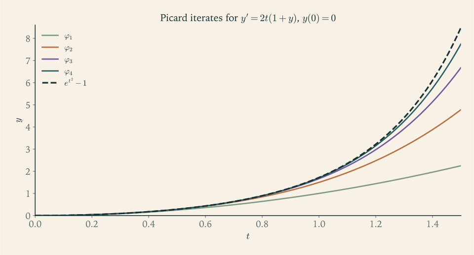
Take \(y'=2t(1+y)\) , \(y(0)=0\) . Starting from \(\varphi_0=0\) :
The pattern is \(\varphi_n(t)=\sum_{k=1}^{n}t^{2k}/k!\) , the partial sums of the series for \(e^{t^2}-1\) . Indeed \(y=e^{t^2}-1\) is the solution, as the linear or the separable method confirms. At \(t=1\) the iterates are \(1\) , \(1.5\) , \(1.6667\) , \(1.7083\) , approaching \(e-1\approx1.7183\) .
3.4 The Picard–Lindelöf theorem
Theorem 3.4 (Picard–Lindelöf). Let \(R\) be the closed rectangle \(\lvert t-t_0\rvert\le a\) , \(\lvert y-y_0\rvert\le b\) . Suppose \(f\) is continuous on \(R\) and Lipschitz in \(y\) on \(R\) with constant \(L\) . Let \(M\) be the maximum of \(\lvert f\rvert\) on \(R\) , and put
with \(h=a\) in the case \(M=0\) . Then the initial value problem \(y'=f(t,y)\) , \(y(t_0)=y_0\) has a solution \(\varphi\) on the interval \(\lvert t-t_0\rvert\le h\) , with graph in \(R\) . It is unique: any solution on a subinterval containing \(t_0\) , with graph in \(R\) , agrees with \(\varphi\) there.
The number \(h\) has a geometric meaning. A solution has slope at most \(M\) in absolute value while it is in \(R\) , so it stays inside the cone \(\lvert y-y_0\rvert\le M\lvert t-t_0\rvert\) , and it cannot leave through the top or bottom of the rectangle before time \(b/M\) has passed. If \(M=0\) then \(f\) vanishes on \(R\) , the constant \(y_0\) is the solution on the whole interval \(\lvert t-t_0\rvert\le a\) , and the proof below covers this case too, with every iterate equal to \(y_0\) .
Proof. Write \(J\) for the interval \(\lvert t-t_0\rvert\le h\) . By Lemma 3.3 it suffices to find a continuous \(\varphi\) on \(J\) , with graph in \(R\) , satisfying the integral equation, and to show there is only one.
The iterates stay in \(R\) . Suppose \(\varphi_n\) is continuous on \(J\) with \(\lvert\varphi_n(t)-y_0\rvert\le b\) . Then \(f(s,\varphi_n(s))\) is defined and continuous, so \(\varphi_{n+1}\) is defined and continuous, and
Since \(\varphi_0=y_0\) has this property, all iterates do, by induction.
The iterates converge. We claim that for all \(n\ge0\) and \(t\in J\) ,
For \(n=0\) this is \(\lvert\varphi_1(t)-y_0\rvert\le M\lvert t-t_0\rvert\) , shown above. If it holds for \(n-1\) , then by the Lipschitz condition
On \(J\)
the right side is at most \(c_n=ML^{n}h^{n+1}/(n+1)!\)
, and \(\sum c_n\)
converges, to \((M/L)(e^{Lh}-1)\)
when \(L>0\)
. The telescoping series \(\varphi_0+\sum_{n\ge0}(\varphi_{n+1}-\varphi_n)\)
therefore converges uniformly on \(J\)
by comparison with \(\sum c_n\)
; call its sum \(\varphi\)
. A uniform limit of continuous functions is continuous (math.real-analysis.uniform-limit-continuity), so \(\varphi\)
is continuous, and \(\lvert\varphi(t)-y_0\rvert\le b\)
because each \(\varphi_n\)
satisfies this.
The limit solves the integral equation. By the Lipschitz condition, \(\lvert f(s,\varphi_n(s))-f(s,\varphi(s))\rvert\le L\sup_J\lvert\varphi_n-\varphi\rvert\) , which tends to \(0\) . Hence \(\int_{t_0}^{t}f(s,\varphi_n(s))\,ds\to\int_{t_0}^{t}f(s,\varphi(s))\,ds\) for each \(t\in J\) . Letting \(n\to\infty\) in \(\varphi_{n+1}(t)=y_0+\int_{t_0}^{t}f(s,\varphi_n(s))\,ds\) gives the integral equation for \(\varphi\) .
Uniqueness. Let \(\psi\) be another solution on a subinterval \(J'\subseteq J\) containing \(t_0\) , with graph in \(R\) . Both satisfy the integral equation, so \(\lvert\varphi(t)-\psi(t)\rvert\le L\bigl\lvert\int_{t_0}^{t}\lvert\varphi-\psi\rvert\,ds\bigr\rvert\) . Let \(K\) be the supremum of \(\lvert\varphi-\psi\rvert\) on \(J'\) , which is at most \(2b\) . Feeding the bound \(K\) into the right side gives \(\lvert\varphi(t)-\psi(t)\rvert\le KL\lvert t-t_0\rvert\) ; feeding that in gives \(KL^2\lvert t-t_0\rvert^2/2\) ; and by induction \(\lvert\varphi(t)-\psi(t)\rvert\le KL^{n}\lvert t-t_0\rvert^{n}/n!\) for every \(n\) . The right side tends to \(0\) as \(n\to\infty\) , so \(\varphi=\psi\) on \(J'\) .
The proof is an instance of a general principle. The operation \(\varphi\mapsto y_0+\int f(s,\varphi)\,ds\)
maps a complete space of continuous functions into itself and, after enough repetitions, shrinks distances by a factor less than one; such a map has exactly one fixed point, reached by iteration from any start. This is the contraction mapping theorem of Functional Analysis (math.functional-analysis.banach-fixed-point), and many existence theorems for differential and integral equations are proved by it. Here the estimates were carried out by hand, which also yields the explicit error bound \(\lvert\varphi-\varphi_n\rvert\le\sum_{k\ge n}c_k\)
.
If the Lipschitz hypothesis is dropped and \(f\) is merely continuous, a solution still exists near \(t_0\) . That is Peano’s theorem; its proof needs a compactness argument and is not given here. Example 3.1 shows that uniqueness is then lost in general. So continuity is the hypothesis for existence, and the Lipschitz condition is the hypothesis for uniqueness.
The theorem is local: it produces a solution on a short interval. Uniqueness, however, extends to any interval on which two solutions are both defined.
Theorem 3.5 (uniqueness on a common interval). Let \(f\) and \(\partial f/\partial y\) be continuous on an open set \(D\) . If \(y_1\) and \(y_2\) are solutions of \(y'=f(t,y)\) on an interval \(I\) , with graphs in \(D\) , and \(y_1(t_0)=y_2(t_0)\) for one \(t_0\in I\) , then \(y_1=y_2\) on all of \(I\) . Equivalently, the graphs of two different solutions never meet.
Proof. Suppose \(y_1(t_1)\ne y_2(t_1)\) for some \(t_1>t_0\) in \(I\) ; the case \(t_1<t_0\) is symmetric. Let \(t^{*}\) be the supremum of the times \(\tau\in[t_0,t_1]\) such that \(y_1=y_2\) on \([t_0,\tau]\) . By continuity \(y_1(t^{*})=y_2(t^{*})\) , so \(t^{*}<t_1\) . The point \((t^{*},y_1(t^{*}))\) lies in \(D\) , and by Lemma 3.2 there is a closed rectangle about it, inside \(D\) , on which \(f\) is Lipschitz. Both \(y_1\) and \(y_2\) are solutions through that point, and for \(t\) near \(t^{*}\) their graphs lie in the rectangle by continuity. The uniqueness part of Theorem 3.4 gives \(y_1=y_2\) on an interval around \(t^{*}\) , which contradicts the definition of \(t^{*}\) .
This is the theorem that Proposition 1.6 borrowed, and it is the reason the curves in Figure 1.1 do not cross.
Example 3.5: How conservative the guaranteed interval is
For \(y'=1+y^2\) , \(y(0)=0\) , take the rectangle \(\lvert t\rvert\le a\) , \(\lvert y\rvert\le b\) . Then \(M=1+b^2\) , the Lipschitz constant is \(L=2b\) by Example 3.3, and
The function \(b/(1+b^2)\) has derivative \((1-b^2)/(1+b^2)^2\) , so it is largest at \(b=1\) , where it equals \(1/2\) . Whatever rectangle is chosen, Theorem 3.4 guarantees a solution only on \(\lvert t\rvert\le1/2\) .
The actual solution is \(y=\tan t\) , which exists on \((-\pi/2,\pi/2)\) , about \(\lvert t\rvert<1.571\) . The theorem’s interval is a third of the truth. This is typical: \(h\) is computed from the worst slope anywhere in the rectangle, while the solution spends most of its time where the slope is smaller. The theorem answers “is there a solution, and is it unique”, not “for how long”. Section 3.6 addresses the second question.
Common mistake. Reading the theorem backward. Picard–Lindelöf says that if \(f\) is Lipschitz then the solution is unique. It does not say that a failure of the Lipschitz condition produces several solutions. For \(y'=1+3y^{2/3}\) , \(y(0)=0\) , the right-hand side fails the Lipschitz condition at \(y=0\) just as in Example 3.1. Yet the solution is unique: the equation is separable with \(h(y)=1+3y^{2/3}\ge1\) , which never vanishes, and part (b) of Theorem 2.2 gives exactly one solution. To prove non-uniqueness one must exhibit two solutions, as Example 3.1 did.
3.5 Grönwall’s inequality and dependence on initial data
A model is useful only if a small error in the initial measurement produces a small error in the prediction. The tool that quantifies this is an inequality for functions that are bounded by their own integral.
Lemma 3.6 (Grönwall’s inequality). Let \(u\) be continuous and nonnegative on \([t_0,t_1]\) , and suppose that for constants \(C\ge0\) and \(L\ge0\) ,
Then \(u(t)\le Ce^{L(t-t_0)}\) on \([t_0,t_1]\) .
Proof. Let \(U(t)=C+L\int_{t_0}^{t}u(s)\,ds\) . Then \(U\) is differentiable with \(U'=Lu\le LU\) and \(U(t_0)=C\) . Therefore
so \(e^{-L(t-t_0)}U(t)\le U(t_0)=C\) , and \(u(t)\le U(t)\le Ce^{L(t-t_0)}\) .
Theorem 3.7 (continuous dependence on the initial value). Let \(f\) be continuous and Lipschitz in \(y\) with constant \(L\) on a set \(D\) , and let \(y_1\) and \(y_2\) be solutions of \(y'=f(t,y)\) on \([t_0,t_1]\) with graphs in \(D\) . Then
Proof. Subtract the integral equations of Lemma 3.3 for the two solutions and apply the Lipschitz condition:
Lemma 3.6 with \(u=\lvert y_1-y_2\rvert\) and \(C=\lvert y_1(t_0)-y_2(t_0)\rvert\) gives the claim.
Taking equal initial values gives \(C=0\) and hence \(y_1=y_2\) : uniqueness once more, by a different argument. For unequal values the theorem says that the gap between two solutions can grow at most exponentially, at the rate \(L\) . The bound cannot be improved in general, because for \(y'=Ly\) the gap between two solutions is exactly \(\lvert y_1(t_0)-y_2(t_0)\rvert e^{L(t-t_0)}\) . But for a particular equation it may be very pessimistic.
Example 3.6: The bound and the truth
For \(y'=\sin y+t\) the derivative of the right side in \(y\) is \(\cos y\) , bounded by \(1\) , so \(L=1\) on the whole plane. Two solutions with \(y_1(0)=1\) and \(y_2(0)=1.01\) therefore satisfy \(\lvert y_2(t)-y_1(t)\rvert\le0.01\,e^{t}\) .
Integrating the two problems numerically gives the actual gaps.
| Time \(t\) | Actual gap | Bound \(0.01\,e^{t}\) |
|---|---|---|
| \(0.5\) | \(0.0115\) | \(0.0165\) |
| \(1\) | \(0.0094\) | \(0.0272\) |
| \(2\) | \(0.0038\) | \(0.0739\) |
The gap first widens and then narrows, because the solutions move into a region where \(\cos y<0\) and neighbouring solutions are pulled together; the bound, which uses only \(\lvert\cos y\rvert\le1\) , cannot see that. Theorem 3.7 guarantees that predictions are stable over a fixed time span. It does not say they are stable forever: if \(L(t-t_0)\) is large, the factor \(e^{L(t-t_0)}\) may exceed any accuracy with which the initial value can be measured.
3.6 How far a solution extends
Theorem 3.4 can be applied again at the end of the interval it produces, extending the solution, and then again. How far can this go?
Definition 3.8 (maximal solution). A solution \(y\) on an open interval \((\alpha,\omega)\) is maximal if it is not the restriction of a solution defined on a strictly larger interval. The interval \((\alpha,\omega)\) is then the maximal interval of existence.
Theorem 3.9 (maximal solutions leave every compact set). Let \(f\) and \(\partial f/\partial y\) be continuous on an open set \(D\) , and let \((t_0,y_0)\in D\) . Then the initial value problem has a unique maximal solution \(y\) on an interval \((\alpha,\omega)\) containing \(t_0\) . If \(K\) is a closed bounded subset of \(D\) , the graph of \(y\) over \([t_0,\omega)\) is not contained in \(K\) , and likewise over \((\alpha,t_0]\) .
Proof. By Theorem 3.5 any two solutions through \((t_0,y_0)\) agree on the intersection of their intervals. So the union of all such solutions is a well-defined function on the union of their intervals, it is a solution, and by construction it cannot be extended. That is the maximal solution, and it is unique.
Suppose the graph over \([t_0,\omega)\) lay in a closed bounded \(K\subseteq D\) . Then \(\omega<\infty\) , and \(\lvert f\rvert\le M\) on \(K\) for some \(M\) , so \(\lvert y'(t)\rvert\le M\) and \(\lvert y(t)-y(s)\rvert\le M\lvert t-s\rvert\) for \(s,t\in[t_0,\omega)\) . By the Cauchy criterion the limit \(y_\omega=\lim_{t\to\omega}y(t)\) exists, and \((\omega,y_\omega)\in K\subseteq D\) because \(K\) is closed. Letting \(t\to\omega\) in the integral equation shows it holds at \(t=\omega\) as well, with \(y(\omega)=y_\omega\) . Since \((\omega,y_\omega)\) is a point of the open set \(D\) , Lemma 3.2 supplies a closed rectangle about it, inside \(D\) , on which \(f\) is Lipschitz in \(y\) . Theorem 3.4 on that rectangle gives a solution \(z\) through \((\omega,y_\omega)\) on some interval \(\lvert t-\omega\rvert\le h\) with \(h>0\) . The function equal to \(y\) on \((\alpha,\omega]\) and to \(z\) on \([\omega,\omega+h)\) is continuous and satisfies the integral equation on \((\alpha,\omega+h)\) , so by Lemma 3.3 it is a solution on a larger interval, contradicting maximality.
In words: a solution can stop only by running out of the region where the equation is well behaved. When \(D\) is a vertical strip \(a<t<b\) , \(y\in\mathbb R\) , a solution that ends at a time \(\omega<b\) cannot remain in any box \([t_0,\omega]\times[-c,c]\) , so it is unbounded as \(t\to\omega\) . (In fact \(\lvert y(t)\rvert\to\infty\) ; proving that requires a slightly longer argument.) Blow-up is the only way for such a solution to end early.
This turns the question of global existence into a question about bounds: if a solution can be shown to stay bounded on every bounded time interval, it exists for all time.
Theorem 3.10 (global existence under linear growth). Let \(f\) and \(\partial f/\partial y\) be continuous for \(a<t<b\) and all real \(y\) , and suppose there are continuous nonnegative functions \(A\) and \(B\) on \((a,b)\) with
Then every maximal solution of \(y'=f(t,y)\) is defined on all of \((a,b)\) .
Proof. Let \(y\) be a maximal solution on \((\alpha,\omega)\) and suppose \(\omega<b\) . On the closed interval \([t_0,\omega]\) the continuous functions \(A\) and \(B\) are bounded by constants \(\bar A\) and \(\bar B\) . From the integral equation, for \(t_0\le t<\omega\) ,
Grönwall’s inequality gives \(\lvert y(t)\rvert\le c\) with \(c=\bigl(\lvert y_0\rvert+\bar B(\omega-t_0)\bigr)e^{\bar A(\omega-t_0)}\) . So the graph over \([t_0,\omega)\) lies in the closed bounded set \([t_0,\omega]\times[-c,c]\) , which is inside the strip. This contradicts Theorem 3.9. Hence \(\omega=b\) , and similarly \(\alpha=a\) .
A linear equation \(y'=-p(t)y+q(t)\) satisfies the hypothesis with \(A=\lvert p\rvert\) and \(B=\lvert q\rvert\) , which recovers the global statement in Theorem 2.3. So does any \(f\) that is bounded, and any \(f\) whose derivative in \(y\) is bounded. The right-hand sides \(y^2\) and \(1+y^2\) grow faster than linearly, and their solutions blow up.
Example 3.7: Trapping a blow-up time without a formula
The Riccati equation \(y'=t^2+y^2\) , \(y(0)=0\) has no elementary solution (Example 2.8). Its maximal solution exists on some \((\alpha,\omega)\) ; we show that \(1<\omega\le1+\pi/2\) .
The solution is positive for \(t>0\) . Since \(y'\ge0\) the solution is nondecreasing, and \(y'(t)\ge t^2>0\) for \(t>0\) , so \(y(t)>0\) for \(t>0\) .
It survives past \(t=1\) . For \(0\le t\le1\) we have \(y'\le1+y^2\) , so \(\dfrac{d}{dt}\arctan y=\dfrac{y'}{1+y^2}\le1\) and \(\arctan y(t)\le t\) . Thus \(y(t)\le\tan t\le\tan1\) on \([0,1]\) as long as the solution exists; being bounded there, it cannot end before \(t=1\) by Theorem 3.9. So \(\omega>1\) .
It ends before \(1+\pi/2\) . For \(t\ge1\) we have \(y'\ge1+y^2\) , so \(\dfrac{d}{dt}\arctan y\ge1\) and
But \(\arctan y<\pi/2\) always. Hence \(t-1<\pi/2\) for every \(t\) in the interval of existence, and \(\omega\le1+\pi/2\approx2.571\) .
A numerical integration places the blow-up at \(\omega\approx2.003\) , inside the bracket. The argument for the upper bound did not use the initial value: every solution of this equation, started anywhere, blows up within time \(\pi\) of the later of its starting time and \(t=1\) . Comparison with an equation that can be solved is the standard way to prove or exclude blow-up.
3.7 Systems and equations of higher order
Everything in this chapter was written for one unknown function, and almost all of it carries over to a system \(\mathbf x'=\mathbf F(t,\mathbf x)\) with \(\mathbf x(t)\in\mathbb R^n\) . Replace absolute values by the Euclidean norm \(\lVert\cdot\rVert\) , replace the rectangle by the set \(\lvert t-t_0\rvert\le a\) , \(\lVert\mathbf x-\mathbf x_0\rVert\le b\) , and call \(\mathbf F\) Lipschitz in \(\mathbf x\) with constant \(L\) if \(\lVert\mathbf F(t,\mathbf x)-\mathbf F(t,\mathbf z)\rVert\le L\lVert\mathbf x-\mathbf z\rVert\) . Integrals of vector functions are taken component by component and satisfy \(\lVert\int\mathbf v\rVert\le\int\lVert\mathbf v\rVert\) . With these changes the integral equation, the Picard iterates and their convergence estimate, the uniqueness argument, Grönwall’s inequality, and the continuation argument are word for word the same.
One step is not the same. Lemma 3.2 obtained a Lipschitz constant from the mean value theorem, and there is no mean value theorem for vector-valued functions: no single intermediate point serves all components at once. The replacement is the fundamental theorem of calculus along the segment from \(\mathbf z\) to \(\mathbf x\) . If the partial derivatives \(\partial F_i/\partial x_j\) are continuous on a set that contains the segment, then for each component
If every partial derivative is at most \(m\) in absolute value on the set, the Cauchy–Schwarz inequality bounds each integrand by \(m\sqrt n\,\lVert\mathbf x-\mathbf z\rVert\) , and therefore \(\lVert\mathbf F(t,\mathbf x)-\mathbf F(t,\mathbf z)\rVert\le nm\,\lVert\mathbf x-\mathbf z\rVert\) . So continuous partial derivatives on an open set again give a local Lipschitz condition, on every closed bounded set of the kind above that lies inside it, since such a set contains the segment between any two of its points with the same \(t\) .
Theorem 3.11 (existence and uniqueness for systems). Let \(\mathbf F\) and all partial derivatives \(\partial F_i/\partial x_j\) be continuous on an open set \(D\) of \((t,\mathbf x)\) -space. Then through each point \((t_0,\mathbf x_0)\in D\) there is exactly one maximal solution of \(\mathbf x'=\mathbf F(t,\mathbf x)\) , \(\mathbf x(t_0)=\mathbf x_0\) , and its graph leaves every closed bounded subset of \(D\) . If \(D\) is a strip \(a<t<b\) , \(\mathbf x\in\mathbb R^n\) , and \(\lVert\mathbf F(t,\mathbf x)\rVert\le A(t)\lVert\mathbf x\rVert+B(t)\) with \(A\) , \(B\) continuous, every maximal solution is defined on all of \((a,b)\) .
The most important application is to linear systems \(\mathbf x'=A(t)\mathbf x+\mathbf g(t)\) with continuous coefficients on an interval \(I\) . The right-hand side has continuous partial derivatives, namely the entries of \(A(t)\) , and satisfies the linear growth bound. So every initial value problem has exactly one solution, defined on all of \(I\) . Since an equation of order \(n\) is a system of \(n\) first-order equations (Section 1.1), this covers the second-order linear equation \(y''+p(t)y'+q(t)y=g(t)\) with data \(y(t_0)\) and \(y'(t_0)\) : one solution, on the whole interval where \(p\) , \(q\) , and \(g\) are continuous. The next chapter is built on that fact.
Exercises
-
For each initial value problem say whether the hypotheses of Theorem 3.4 hold on some rectangle about the initial point, giving a reason: (a) \(y'=t+y^2\) , \(y(0)=0\) ; (b) \(y'=\sqrt{\lvert y\rvert}\) , \(y(0)=0\) ; (c) \(y'=\sqrt{\lvert y\rvert}\) , \(y(0)=1\) ; (d) \(y'=\lvert y\rvert\) , \(y(0)=0\) ; (e) \(y'=y/t\) , \(y(0)=1\) .
Answer
(a) Yes: \(f=t+y^2\) and \(f_y=2y\) are continuous everywhere. (b) No: \(f\) is continuous, but \(\sqrt{\lvert y\rvert}/\lvert y\rvert\) is unbounded near \(0\) , so no Lipschitz constant exists on a rectangle about \((0,0)\) ; a solution exists but is not unique. (c) Yes: on \(\lvert y-1\rvert\le\tfrac12\) the derivative \(1/(2\sqrt y)\) is bounded. (d) Yes: \(\lvert y\rvert\) is Lipschitz with constant \(1\) ; the unique solution is \(y=0\) . (e) No: \(y/t\) is not defined at \(t=0\) , and there is in fact no solution, since \(ty'=y\) forces \(y(0)=0\) .
-
Compute the Picard iterates \(\varphi_1,\varphi_2,\varphi_3\) for \(y'=y\) , \(y(0)=1\) and for \(y'=t+y\) , \(y(0)=0\) , and identify the function to which each sequence converges.
Answer
For \(y'=y\) : \(\varphi_1=1+t\) , \(\varphi_2=1+t+\tfrac12t^2\) , \(\varphi_3=1+t+\tfrac12t^2+\tfrac16t^3\) , converging to \(e^{t}\) . For \(y'=t+y\) : \(\varphi_1=\tfrac12t^2\) , \(\varphi_2=\tfrac12t^2+\tfrac16t^3\) , \(\varphi_3=\tfrac12t^2+\tfrac16t^3+\tfrac1{24}t^4\) , converging to \(e^{t}-1-t\) .
-
For \(y'=2\sqrt{\lvert y\rvert}\) , \(y(0)=0\) , verify that for each \(c\ge0\) the function equal to \(0\) for \(t\le c\) and to \((t-c)^2\) for \(t>c\) is a solution on \(\mathbb R\) , checking differentiability at \(t=c\) ; then describe a solution that is negative for \(t<-1\) , zero on \([-1,2]\) , and positive for \(t>2\) .
Solution
Fix \(c\ge0\) and call the function \(y_c\) . For \(t<c\) it is identically \(0\) , so \(y_c'=0=2\sqrt{\lvert0\rvert}\) . For \(t>c\) , \(y_c=(t-c)^2\) gives \(y_c'=2(t-c)\) and \(2\sqrt{\lvert y_c\rvert}=2\lvert t-c\rvert=2(t-c)\) because \(t-c>0\) . At \(t=c\) the left difference quotient is \(0\) and the right one is \((t-c)^2/(t-c)=t-c\to0\) , so \(y_c\) is differentiable at \(c\) with derivative \(0\) , which equals \(2\sqrt{\lvert y_c(c)\rvert}=0\) . Hence \(y_c\) is a solution on \(\mathbb R\) , and \(y_c(0)=0\) since \(0\le c\) .
For the second part, a solution may also arrive at zero from below. Put
\[ y(t)=\begin{cases}-(t+1)^2,& t<-1,\\ 0,& -1\le t\le2,\\ (t-2)^2,& t>2.\end{cases} \]For \(t<-1\) , \(y'=-2(t+1)=2\lvert t+1\rvert\) because \(t+1<0\) , and \(2\sqrt{\lvert y\rvert}=2\lvert t+1\rvert\) . The matching at \(t=-1\) is as before. So this is a solution, negative before \(-1\) , zero on \([-1,2]\) , positive after \(2\) , and it satisfies \(y(0)=0\) . Every solution is nondecreasing since \(y'\ge0\) , and the general solution through the origin has this shape, with arbitrary departure times on both sides.
-
Find the smallest Lipschitz constant in \(y\) for \(f(t,y)=ty^2\) on the rectangle \(\lvert t\rvert\le2\) , \(\lvert y\rvert\le3\) and for \(f(t,y)=\sin(ty)\) on the strip \(\lvert t\rvert\le5\) , and show that \(f(t,y)=y^{1/3}\) is not Lipschitz on any interval containing \(y=0\) .
Answer
For \(ty^2\) : \(\lvert f_y\rvert=\lvert2ty\rvert\le12\) on the rectangle, with equality at a corner, so \(L=12\) . For \(\sin(ty)\) : \(\lvert f_y\rvert=\lvert t\cos(ty)\rvert\le5\) , and the value \(5\) is attained at \(t=5\) , \(y=0\) , so \(L=5\) . For \(y^{1/3}\) : the quotient \(\lvert y^{1/3}-0\rvert/\lvert y-0\rvert=\lvert y\rvert^{-2/3}\) is unbounded as \(y\to0\) .
-
For \(y'=y^2\) , \(y(0)=1\) and the rectangle \(\lvert t\rvert\le a\) , \(\lvert y-1\rvert\le b\) , compute \(M\) and the guaranteed half-length \(h\) , find the choice of \(b\) that makes \(h\) largest, and compare with the true maximal interval.
Solution
On the rectangle the largest value of \(\lvert f\rvert=y^2\) occurs at the top edge \(y=1+b\) , so \(M=(1+b)^2\) , and
\[ h=\min\Bigl(a,\frac{b}{(1+b)^2}\Bigr). \]The function \(g(b)=b/(1+b)^2\) has derivative \(g'(b)=\dfrac{(1+b)^2-2b(1+b)}{(1+b)^4}=\dfrac{1-b}{(1+b)^3}\) , which is positive for \(b<1\) and negative for \(b>1\) . So \(g\) is largest at \(b=1\) , where \(g(1)=1/4\) . Taking \(b=1\) and any \(a\ge1/4\) gives the best guaranteed half-length \(h=1/4\) : Theorem 3.4 promises a solution on \([-1/4,1/4]\) .
The true solution is \(y=1/(1-t)\) on the maximal interval \((-\infty,1)\) . To the right the theorem delivers a quarter of the available interval, and to the left it delivers \(1/4\) of an infinite one. The estimate is poor on the left because the rectangle is symmetric in \(t\) and \(M\) is governed by the top edge, which the solution approaches only for \(t>0\) ; going left the solution decreases toward \(0\) and the slopes become small.
-
Find the maximal interval of existence of the solution of \(y'=y^2\) , \(y(0)=y_0\) for every real \(y_0\) , treating \(y_0>0\) , \(y_0=0\) , and \(y_0<0\) separately, and sketch the three kinds of solution.
Answer
For \(y_0\ne0\) the solution is \(y=y_0/(1-y_0t)\) . If \(y_0>0\) the interval is \((-\infty,1/y_0)\) and \(y\to+\infty\) at the right end. If \(y_0<0\) the interval is \((1/y_0,\infty)\) and \(y\to-\infty\) at the left end. If \(y_0=0\) the solution is \(y=0\) on \(\mathbb R\) .
-
For the leaking bucket \(h'=-k\sqrt h\) with \(k>0\) , show that the condition \(h(T)=0\) is satisfied by infinitely many solutions on \(t\le T\) , explain why Theorem 3.4 does not apply at the point \((T,0)\) , and prove that nevertheless every solution with \(h(T)=0\) is zero for all \(t\ge T\) .
Solution
Many solutions. For any \(c\le T\) define \(h_c(t)=\tfrac{k^2}{4}(c-t)^2\) for \(t<c\) and \(h_c(t)=0\) for \(t\ge c\) . For \(t<c\) , \(h_c'=-\tfrac{k^2}{2}(c-t)\) and \(-k\sqrt{h_c}=-k\cdot\tfrac k2(c-t)\) , which agree. At \(t=c\) both one-sided derivatives are \(0\) . So \(h_c\) is a solution with \(h_c(T)=0\) , and different values of \(c\) give different solutions on \(t\le T\) : the bucket emptied at time \(c\) , and any \(c\le T\) is possible.
Why the theorem is silent. The right-hand side \(-k\sqrt h\) has difference quotient \(k\sqrt h/h=k/\sqrt h\) against \(h=0\) , unbounded as \(h\to0^{+}\) . It is not Lipschitz on any rectangle containing \((T,0)\) , and the function is not even defined for \(h<0\) .
Forward uniqueness. Let \(h\) be any solution with \(h(T)=0\) . Solutions take values \(h\ge0\) , where the equation is defined, and \(h'=-k\sqrt h\le0\) , so \(h\) is nonincreasing. For \(t\ge T\) this gives \(h(t)\le h(T)=0\) , and with \(h\ge0\) we get \(h(t)=0\) . So the future of an empty bucket is determined, while its past is not. Uniqueness can hold in one time direction and fail in the other.
-
Let \(u\) be continuous and nonnegative on \([t_0,t_1]\) with \(u(t)\le L\int_{t_0}^{t}u(s)\,ds\) for all \(t\) . Prove directly, by the iteration used in the uniqueness part of Theorem 3.4 and without quoting Grönwall’s inequality, that \(u\) is identically zero.
Solution
Let \(K\) be the maximum of \(u\) on \([t_0,t_1]\) , which exists because \(u\) is continuous on a closed bounded interval. We show by induction that
\[ u(t)\le\frac{K\,L^{n}(t-t_0)^{n}}{n!}\quad\text{for all }t\in[t_0,t_1]\text{ and all }n\ge0 . \]For \(n=0\) this is \(u\le K\) . If it holds for \(n\) , substitute it into the hypothesis:
\[ u(t)\le L\int_{t_0}^{t}\frac{KL^{n}(s-t_0)^{n}}{n!}\,ds=\frac{KL^{n+1}(t-t_0)^{n+1}}{(n+1)!}. \]So it holds for \(n+1\) . For fixed \(t\) , the right side is \(K\) times the general term of the convergent exponential series for \(e^{L(t-t_0)}\) , so it tends to \(0\) as \(n\to\infty\) . Since \(0\le u(t)\) is bounded above by a quantity tending to zero, \(u(t)=0\) .
This is exactly Grönwall’s inequality in the case \(C=0\) , and applying it to \(u=\lvert y_1-y_2\rvert\) for two solutions with the same initial value reproves uniqueness.
-
A student argues: “The function \(y^2\) has a continuous derivative everywhere, so by Picard–Lindelöf the solution of \(y'=y^2\) , \(y(0)=1\) exists for all \(t\) .” Identify exactly which statement of the theorem has been misread, and explain in terms of \(M\) and \(b\) why repeated application of the theorem does not reach \(t=1\) .
Solution
The theorem’s conclusion is local: a solution exists on \(\lvert t-t_0\rvert\le h\) with \(h=\min(a,b/M)\) . The student has read “exists” as “exists for all \(t\) ”. Continuity of \(f\) and \(f_y\) everywhere means the theorem can be applied at every point, not that one application covers every time.
To see why repetition does not help, apply the theorem at a point \((t_k,y_k)\) on the solution, with \(y_k>0\) . On a rectangle of half-height \(b\) the bound is \(M=(y_k+b)^2\) , so the step is at most \(b/(y_k+b)^2\le1/(4y_k)\) , the maximum being at \(b=y_k\) . The true solution is \(y=1/(1-t)\) , so \(y_k=1/(1-t_k)\) and the step from \(t_k\) is at most \((1-t_k)/4\) . Each application therefore covers at most a quarter of the remaining distance to \(t=1\) : after \(n\) steps the distance left is at least \((3/4)^n\) , which is positive for every \(n\) . The guaranteed intervals shrink geometrically because \(M\) grows as the solution does, and their total length never reaches \(1\) . That is consistent with Theorem 3.9: the solution ends by leaving every bounded set.
-
Decide which of these equations have all solutions defined for all \(t\) , citing Theorem 3.10 or exhibiting a solution that blows up: (a) \(y'=e^{t}\cos y\) ; (b) \(y'=ty+\sin y\) ; (c) \(y'=y^3\) .
Hint
(a) \(\lvert f\rvert\le e^{t}\) , so take \(A=0\) and \(B=e^{t}\) . (b) \(\lvert f\rvert\le\lvert t\rvert\,\lvert y\rvert+1\) . (c) Separate variables; the solution with \(y(0)=y_0>0\) is \(y_0/\sqrt{1-2y_0^2t}\) , which blows up at \(t=1/(2y_0^2)\) .
-
Solve \(y'=e^{y}\) , \(y(0)=0\) explicitly, find its maximal interval of existence, and say which hypothesis of Theorem 3.10 fails.
Answer
Separating, \(-e^{-y}=t-1\) , so \(y=-\ln(1-t)\) on \((-\infty,1)\) . The right-hand side \(e^{y}\) is not bounded by \(A\lvert y\rvert+B\) for large positive \(y\) .
-
Two solutions of \(y'=\cos y+t^2\) start at \(y(0)=0\) and \(y(0)=0.001\) . Use Theorem 3.7 to bound their difference at \(t=2\) , and then show that for the equation \(y'=3y\) the corresponding bound holds with equality.
Answer
Here \(\lvert\partial f/\partial y\rvert=\lvert\sin y\rvert\le1\) , so \(L=1\) and the difference at \(t=2\) is at most \(0.001\,e^{2}\approx0.0074\) . For \(y'=3y\) the solutions are \(y_0e^{3t}\) , so the difference of two is \(\lvert\Delta y_0\rvert e^{3t}\) , which is the bound of Theorem 3.7 with \(L=3\) .
-
Prove by induction that the Picard iterates for \(y'=ky\) , \(y(0)=1\) are \(\varphi_n(t)=\sum_{j=0}^{n}(kt)^j/j!\) , and deduce from Theorem 3.4 a proof that this series converges to a solution of the equation.
Hint
The induction step is \(\varphi_{n+1}=1+\int_0^tk\,\varphi_n(s)\,ds\) , integrated term by term. Theorem 3.4 applies on any rectangle, and its proof shows the iterates converge uniformly to the solution.
-
Let \(y\) be the maximal solution of \(y'=(1+t^2)\,y\,(1-y)\) with \(0<y(0)<1\) . Use Theorem 3.5 to show that \(0<y(t)<1\) for all \(t\) in its interval of existence, and then Theorem 3.9 to conclude that the interval is all of \(\mathbb R\) .
Solution
The right-hand side \(f(t,y)=(1+t^2)y(1-y)\) and its derivative in \(y\) are polynomials, hence continuous on the whole plane, so Theorems 3.5 and 3.9 apply with \(D=\mathbb R^2\) .
The constant functions \(y=0\) and \(y=1\) are solutions on \(\mathbb R\) , since \(f(t,0)=f(t,1)=0\) for every \(t\) . By Theorem 3.5 the graphs of different solutions never meet. Our solution starts strictly between \(0\) and \(1\) . If it took the value \(1\) at some time, or the value \(0\) , its graph would meet the graph of a constant solution without being equal to it, which is impossible. If it took a value above \(1\) or below \(0\) , the intermediate value theorem would force it to take the value \(1\) or \(0\) first. Hence \(0<y(t)<1\) throughout the interval of existence \((\alpha,\omega)\) .
Suppose \(\omega<\infty\) . Then the graph over \([0,\omega)\) lies in the closed bounded set \([0,\omega]\times[0,1]\) , contradicting Theorem 3.9. So \(\omega=\infty\) , and similarly \(\alpha=-\infty\) . Note that Theorem 3.10 does not apply directly, since \(f\) grows quadratically in \(y\) ; the constant solutions act as barriers and supply the bound instead.
-
Write the pendulum equation \(\theta''=-\sin\theta\) as a system for \((x_1,x_2)=(\theta,\theta')\) , show that the right-hand side is Lipschitz with constant \(1\) on the whole plane using \(\lvert\sin a-\sin b\rvert\le\lvert a-b\rvert\) , and conclude that every solution exists for all time.
Hint
The system is \(x_1'=x_2\) , \(x_2'=-\sin x_1\) . Estimate \(\lVert\mathbf F(\mathbf x)-\mathbf F(\mathbf z)\rVert^2=(x_2-z_2)^2+(\sin x_1-\sin z_1)^2\) . For global existence use the growth bound \(\lVert\mathbf F(\mathbf x)\rVert\le\lVert\mathbf x\rVert+1\) in Theorem 3.11.
-
Compute the Picard iterates \(\boldsymbol\varphi_1,\boldsymbol\varphi_2,\boldsymbol\varphi_3,\boldsymbol\varphi_4\) for the system \(x'=y\) , \(y'=-x\) with \((x(0),y(0))=(1,0)\) , where each iterate is a pair of functions, and recognise the limit.
Answer
\(\boldsymbol\varphi_1=(1,-t)\) , \(\boldsymbol\varphi_2=(1-\tfrac12t^2,-t)\) , \(\boldsymbol\varphi_3=(1-\tfrac12t^2,-t+\tfrac16t^3)\) , \(\boldsymbol\varphi_4=(1-\tfrac12t^2+\tfrac1{24}t^4,-t+\tfrac16t^3)\) . These are Taylor polynomials of \((\cos t,-\sin t)\) , the solution.
-
For \(y'=t^2+y^2\) let \(\omega(y_0)\) be the blow-up time of the solution with \(y(0)=y_0\) . Explain why solutions with different initial values never cross, and deduce that \(\omega\) is a nonincreasing function of \(y_0\) .
Solution
The function \(f(t,y)=t^2+y^2\) and its derivative \(2y\) are continuous on the plane, so by Theorem 3.5 two solutions that agree at one time agree on their whole common interval. Take \(y_0<z_0\) and let \(y\) and \(z\) be the corresponding maximal solutions. On the common part of their intervals to the right of \(0\) they can never be equal. The difference \(z-y\) is continuous, positive at \(t=0\) , and never zero, so by the intermediate value theorem it stays positive: \(y(t)<z(t)\) wherever both exist.
Now compare blow-up times. Suppose, for contradiction, that \(\omega(y_0)<\omega(z_0)\) . Then \(z\) is defined and continuous on the closed interval \([0,\omega(y_0)]\) , hence bounded there by some constant \(c\) . On \([0,\omega(y_0))\) we have \(y(0)\le y(t)<z(t)\le c\) , where the lower bound holds because \(y'\ge0\) . So the graph of \(y\) over \([0,\omega(y_0))\) lies in a closed bounded rectangle, contradicting Theorem 3.9. Therefore \(\omega(y_0)\ge\omega(z_0)\) whenever \(y_0<z_0\) : a larger start cannot blow up later.
-
Solve \(y'=c\,(1+y^2)\cos t\) , \(y(0)=0\) for a constant \(c>0\) . Show that the solution exists for all \(t\) when \(c<\pi/2\) and blows up in finite time when \(c\ge\pi/2\) , and find the blow-up time for \(c=2\) .
Solution
The equation is separable with \(h(y)=1+y^2\) , which never vanishes, so by Theorem 2.2 the solution is given by
\[ \arctan y=c\int_0^t\cos s\,ds=c\sin t,\qquad y(t)=\tan(c\sin t), \]valid as long as \(c\sin t\) stays in the range \((-\pi/2,\pi/2)\) of the arctangent.
If \(c<\pi/2\) , then \(\lvert c\sin t\rvert\le c<\pi/2\) for every \(t\) , so the formula defines a solution on all of \(\mathbb R\) ; it is periodic and bounded by \(\tan c\) . Theorem 3.10 could not have predicted this, since the right side grows quadratically in \(y\) .
If \(c\ge\pi/2\) , then \(c\sin t\) increases from \(0\) and reaches \(\pi/2\) at the first positive time with \(\sin t=\pi/(2c)\) , namely
\[ \omega=\arcsin\frac{\pi}{2c}, \]and \(y\to+\infty\) there. For \(c=2\) this is \(\arcsin(\pi/4)\approx0.903\) . By symmetry the solution also blows up, to \(-\infty\) , at \(t=-\omega\) . The threshold \(c=\pi/2\) separates global existence from blow-up for one and the same smooth nonlinearity; what decides the matter is whether the accumulated forcing \(\int\cos\) is large enough to carry \(\arctan y\) to \(\pi/2\) .