Chapter 2: First-Order Method Choice

Date: Oct 2, 2026

Here are three equations that look almost alike:

\[ y'=ty,\qquad y'=t+y,\qquad y'=t^2+y^2 . \]

The first can be solved in one line by putting everything involving \(y\) on one side. That device fails for the second, which nevertheless has an explicit solution found by a different idea. The third has no solution expressible through elementary functions at all, although the direction-field methods of Chapter 1 describe its solutions perfectly well. Nothing in the appearance of the three right-hand sides announces these differences.

There is no general method for solving \(y'=f(t,y)\) in closed form. What exists is a short list of structures, each with its own method and its own conditions of validity. Solving a first-order equation is therefore first an act of recognition. This chapter treats the four structures that account for nearly every first-order equation solved by hand, separable, linear, exact, and reducible by substitution, and for each one it states precisely what the method proves and where it can silently lose a solution.

2.1 Separable equations

Definition 2.1 (separable equation). A first-order equation is separable if it can be written

\[ y'=g(t)\,h(y) \]

with \(g\) a function of \(t\) alone and \(h\) a function of \(y\) alone.

The informal recipe is familiar: write \(dy/h(y)=g(t)\,dt\) and integrate both sides. The recipe treats \(dy/dt\) as a fraction, which it is not, so it needs a justification; and it divides by \(h(y)\) , which may be zero. The following theorem deals with both points.

Theorem 2.2 (solution of a separable equation). Let \(g\) be continuous on an open interval \(I\) and let \(h\) be continuous on an open interval \(J\) .

(a) If \(h(c)=0\) for some \(c\in J\) , the constant function \(y(t)=c\) is a solution on \(I\) .

(b) Suppose \(h(y)\ne 0\) for every \(y\in J\) , and let \(t_0\in I\) , \(y_0\in J\) . Put

\[ G(t)=\int_{t_0}^{t}g(s)\,ds,\qquad H(y)=\int_{y_0}^{y}\frac{du}{h(u)} . \]

Then a function \(y\) with values in \(J\) , defined on an open interval \(I'\subseteq I\) containing \(t_0\) , is a solution of \(y'=g(t)h(y)\) , \(y(t_0)=y_0\) if and only if

\[ H\bigl(y(t)\bigr)=G(t)\quad\text{for all }t\in I' . \]

Such a solution exists on some interval \(I'\) , and any two of them agree where both are defined.

Proof. Part (a) is immediate: \(y'=0=g(t)h(c)\) .

For (b), note that \(H\) is differentiable on \(J\) with \(H'(y)=1/h(y)\) by the fundamental theorem of calculus. Since \(h\) is continuous and never zero on the interval \(J\) , it has one sign there, so \(H\) is strictly monotone and has a differentiable inverse on its range, which is an open interval containing \(H(y_0)=0\) .

If \(y\) is a solution with values in \(J\) , the chain rule gives

\[ \frac{d}{dt}H\bigl(y(t)\bigr)=\frac{y'(t)}{h(y(t))}=g(t)=G'(t), \]

and \(H(y(t_0))=0=G(t_0)\) , so \(H(y(t))=G(t)\) on \(I'\) . Conversely, if \(H(y(t))=G(t)\) on \(I'\) then \(y(t)=H^{-1}(G(t))\) is differentiable, and differentiating the identity gives \(y'(t)/h(y(t))=g(t)\) ; also \(H(y(t_0))=0\) forces \(y(t_0)=y_0\) because \(H\) is one-to-one.

Because \(G\) is continuous with \(G(t_0)=0\) , the values \(G(t)\) lie in the range of \(H\) for \(t\) near \(t_0\) , so \(y=H^{-1}\circ G\) is defined on some open interval about \(t_0\) ; this proves existence. Uniqueness holds because any solution with values in \(J\) must equal \(H^{-1}\circ G\) .

Three remarks. First, the theorem gives the solution implicitly, as the relation \(H(y)=G(t)\) ; solving that relation for \(y\) is a separate algebraic step that is sometimes impossible in elementary terms. Second, the constant solutions of part (a) are not contained in the relation of part (b), because the division that produces \(H\) is not allowed at a zero of \(h\) . They must be collected separately, before dividing. Third, the uniqueness statement is restricted to solutions that stay in an interval where \(h\ne 0\) . What can happen when a solution reaches a zero of \(h\) is one of the subjects of Chapter 3.

Example 2.1: Three initial conditions, three kinds of answer

Solve \(y'=ty^2\) with (i) \(y(0)=1\) , (ii) \(y(0)=0\) , (iii) \(y(0)=-1\) .

Here \(g(t)=t\) and \(h(y)=y^2\) . The only zero of \(h\) is \(y=0\) , so \(y(t)=0\) is a constant solution on \(\mathbb R\) ; that settles (ii).

On either interval \(J=(0,\infty)\) or \(J=(-\infty,0)\) we may divide. An antiderivative of \(1/y^2\) is \(-1/y\) , so the solutions with \(y\ne 0\) satisfy

\[ -\frac1y=\frac{t^2}{2}+C . \]

For (i), \(y(0)=1\) gives \(C=-1\) , hence \(-1/y=(t^2-2)/2\) and

\[ y(t)=\frac{2}{2-t^2},\qquad -\sqrt2<t<\sqrt2 . \]

The interval is the largest one containing \(t_0=0\) on which the denominator does not vanish; the solution tends to \(+\infty\) at both ends.

For (iii), \(y(0)=-1\) gives \(C=1\) and

\[ y(t)=-\frac{2}{2+t^2},\qquad t\in\mathbb R . \]

This solution exists for all time and tends to \(0\) as \(t\to\pm\infty\) without ever reaching it.

Three starting values a short distance apart give a solution that blows up in finite time, a solution that is identically zero, and a solution that lives forever. No single formula \(y=-2/(t^2+2C)\) covers the three: the zero solution corresponds to no finite \(C\) .

Example 2.2: The logistic equation

Solve \(y'=y(1-y)\) , \(y(0)=1/4\) , and find when \(y\) reaches \(1/2\) .

The zeros of \(h(y)=y(1-y)\) give the equilibrium solutions \(y=0\) and \(y=1\) . The initial value lies in \(J=(0,1)\) , where \(h>0\) . By partial fractions,

\[ \frac{1}{y(1-y)}=\frac1y+\frac{1}{1-y},\qquad \int\frac{dy}{y(1-y)}=\ln\frac{y}{1-y}\quad(0<y<1). \]

The relation \(H(y)=G(t)\) becomes \(\ln\dfrac{y}{1-y}=t+C\) , and \(y(0)=1/4\) gives \(C=\ln(1/3)\) . Exponentiating, \(y/(1-y)=e^{t}/3\) , and solving for \(y\) ,

\[ y(t)=\frac{e^{t}}{3+e^{t}}=\frac{1}{1+3e^{-t}} . \]

The formula is defined for all \(t\) and stays strictly between \(0\) and \(1\) , so the solution never leaves \(J\) and the interval of existence is \(\mathbb R\) . It increases from \(0\) toward \(1\) , in agreement with the phase line. It equals \(1/2\) when \(3e^{-t}=1\) , at \(t=\ln 3\approx 1.099\) .

Common mistake. Dividing by \(h(y)\) and reporting only what the integration produces. For \(y'=y(1-y)\) the family obtained by separation, \(y=1/(1+Ae^{-t})\) , contains the equilibrium \(y=1\) (take \(A=0\) ) but not the equilibrium \(y=0\) . A student who concludes that the initial value problem with \(y(0)=0\) “has no solution because no \(A\) works” has discarded the solution at the first step. List the zeros of \(h\) and the corresponding constant solutions before dividing.

2.2 Linear equations

The equation \(y'=t+y\) is not separable: no factorization \(t+y=g(t)h(y)\) exists, since such a product vanishes on a union of horizontal and vertical lines while \(t+y\) vanishes on a slanted one. It is, however, linear, and linear equations have a complete theory.

Theorem 2.3 (first-order linear equations). Let \(p\) and \(q\) be continuous on an open interval \(I\) , and let \(t_0\in I\) . For every real \(y_0\) the initial value problem

\[ y'+p(t)\,y=q(t),\qquad y(t_0)=y_0 \]

has exactly one solution, and it is defined on all of \(I\) . With the integrating factor \(\mu(t)=\exp\Bigl(\int_{t_0}^{t}p(s)\,ds\Bigr)\) it is

\[ y(t)=\frac{1}{\mu(t)}\Bigl(y_0+\int_{t_0}^{t}\mu(s)\,q(s)\,ds\Bigr). \]

Proof. The function \(\mu\) is positive and differentiable on \(I\) with \(\mu'=p\mu\) and \(\mu(t_0)=1\) . For any differentiable \(y\) , the product rule gives

\[ (\mu y)'=\mu y'+\mu'y=\mu\,(y'+py). \]

Since \(\mu\) is never zero, \(y\) satisfies \(y'+py=q\) on \(I\) if and only if \((\mu y)'=\mu q\) on \(I\) . By the fundamental theorem of calculus, that holds together with \(y(t_0)=y_0\) if and only if \(\mu(t)y(t)=y_0+\int_{t_0}^{t}\mu q\) for all \(t\in I\) . Dividing by \(\mu\) gives the formula, which therefore describes the one and only solution; it is defined wherever \(p\) and \(q\) are continuous, that is, on all of \(I\) .

The proof is the method: multiply the equation in normal form by \(\mu=e^{\int p}\) and the left side becomes the derivative of \(\mu y\) . Any antiderivative of \(p\) may be used in the exponent, since changing it multiplies \(\mu\) by a constant that cancels.

The theorem says three things that are false for nonlinear equations in general, and Example 2.1 violated all three. The solution exists on the whole interval where the coefficients are continuous; it cannot blow up earlier. The interval of existence can be read from the equation before solving. And one formula with one constant contains every solution. Writing the formula as

\[ y(t)=\underbrace{\frac{1}{\mu(t)}\int_{t_0}^{t}\mu q}_{\text{one particular solution}}\;+\;\underbrace{\frac{y_0}{\mu(t)}}_{\text{solution of }y'+py=0} \]

shows the structure that recurs for every linear equation in this book: a particular solution plus the general solution of the homogeneous equation.

Example 2.3: A singular coefficient fixes the interval

Solve \(ty'+2y=4t^2\) , \(y(1)=2\) .

Divide by \(t\) to reach normal form: \(y'+\dfrac2t\,y=4t\) . The coefficient \(p(t)=2/t\) is continuous on \((-\infty,0)\) and on \((0,\infty)\) ; the initial time \(t_0=1\) lies in \((0,\infty)\) , so Theorem 2.3 promises a unique solution on \((0,\infty)\) before any computation.

An integrating factor is \(\mu=\exp(2\ln t)=t^2\) . Multiplying,

\[ (t^2y)'=4t^3,\qquad t^2y=t^4+C,\qquad y=t^2+\frac{C}{t^2}. \]

The condition \(y(1)=2\) gives \(C=1\) :

\[ y(t)=t^2+\frac{1}{t^2},\qquad t>0 . \]

Check: \(ty'+2y=t\,(2t-2t^{-3})+2t^2+2t^{-2}=4t^2\) . The solution is unbounded as \(t\to 0^{+}\) , which is consistent with the theorem, since \(0\) is not in the interval where \(p\) is continuous.

Example 2.4: Response to a sinusoidal input

Solve \(y'+2y=5\cos t\) , \(y(0)=0\) , and describe the behaviour for large \(t\) .

Here \(\mu=e^{2t}\) and \((e^{2t}y)'=5e^{2t}\cos t\) . Integrating by parts twice, or checking by differentiation,

\[ \int 5e^{2t}\cos t\,dt=e^{2t}\,(2\cos t+\sin t)+C . \]

Hence \(y=2\cos t+\sin t+Ce^{-2t}\) , and \(y(0)=0\) gives \(C=-2\) :

\[ y(t)=2\cos t+\sin t-2e^{-2t}. \]

The term \(-2e^{-2t}\) is the transient: it carries the initial condition and is below one percent of its starting size after \(t=\ln(100)/2\approx 2.3\) . What remains is the steady response \(2\cos t+\sin t\) , which does not depend on \(y(0)\) at all. Writing it as a single cosine,

\[ 2\cos t+\sin t=\sqrt5\,\cos(t-\phi),\qquad \phi=\arctan\tfrac12\approx 0.464, \]

shows that the response has the same frequency as the input, amplitude \(\sqrt5\approx 2.24\) in place of the input’s \(5\) , and lags behind the input by \(0.464\) radians. Amplitude ratio and phase lag are the two numbers that describe how a linear system responds to an oscillating input; Chapter 5 computes them for second-order equations, where they produce resonance.

Common mistake. Computing the integrating factor before putting the equation in normal form. For \(2y'+6y=e^{-t}\) , reading off “\(p=6\) ” gives \(\mu=e^{6t}\) , and then \((\mu y)'\) is not the left side of anything. The coefficient of \(y'\) must be \(1\) first: \(y'+3y=\tfrac12e^{-t}\) , \(\mu=e^{3t}\) .

2.3 Exact equations

A first-order equation can be written symmetrically as

\[ M(x,y)\,dx+N(x,y)\,dy=0, \]

which is shorthand for \(M(x,y)+N(x,y)\,y'=0\) when \(y\) is regarded as a function of \(x\) . In this section the independent variable is called \(x\) , since the symmetric form treats the two variables alike.

Suppose there is a function \(\Phi(x,y)\) whose partial derivatives are \(\Phi_x=M\) and \(\Phi_y=N\) . For a differentiable function \(y(x)\) , the chain rule for a function of two variables along a curve (math.multivariable-calculus.total-derivative-chain-rule) gives

\[ \frac{d}{dx}\Phi\bigl(x,y(x)\bigr)=\Phi_x+\Phi_y\,y'=M+N\,y' . \]

So \(y\) is a solution exactly when \(\Phi(x,y(x))\) is constant: the solution curves are pieces of the level curves \(\Phi(x,y)=C\) .

Definition 2.4 (exact equation, potential). The equation \(M\,dx+N\,dy=0\) is exact on a region \(R\) of the plane if there is a continuously differentiable function \(\Phi\) on \(R\) with \(\Phi_x=M\) and \(\Phi_y=N\) . Such a \(\Phi\) is a potential for the equation.

Theorem 2.5 (test for exactness). Let \(M\) and \(N\) have continuous first partial derivatives on an open rectangle \(R\) . The equation \(M\,dx+N\,dy=0\) is exact on \(R\) if and only if

\[ \frac{\partial M}{\partial y}=\frac{\partial N}{\partial x}\quad\text{on }R . \]

Proof. If a potential exists, then \(M_y=\Phi_{xy}\) and \(N_x=\Phi_{yx}\) , and these mixed partial derivatives are equal because they are continuous.

Conversely, assume \(M_y=N_x\) on \(R\) and fix a point \((x_0,y_0)\in R\) . Define

\[ \Phi(x,y)=\int_{x_0}^{x}M(s,y_0)\,ds+\int_{y_0}^{y}N(x,u)\,du . \]

Both integrals are over segments that lie in \(R\) because \(R\) is a rectangle. The first term does not depend on \(y\) , so \(\Phi_y=N(x,y)\) by the fundamental theorem of calculus. For \(\Phi_x\) , differentiate the first term by the fundamental theorem and the second under the integral sign, which is permitted because \(N_x\) is continuous:

\[ \Phi_x(x,y)=M(x,y_0)+\int_{y_0}^{y}N_x(x,u)\,du=M(x,y_0)+\int_{y_0}^{y}M_y(x,u)\,du=M(x,y). \]

The last step is the fundamental theorem again, applied to \(u\mapsto M(x,u)\) .

The proof is also the procedure: integrate \(M\) with respect to \(x\) , then adjust by a function of \(y\) alone so that the \(y\) -derivative comes out as \(N\) .

Example 2.5: A potential, a level curve, and where the solution stops

Solve \((2xy+3)\,dx+(x^2+4y)\,dy=0\) with \(y(0)=1\) .

Test. \(M_y=2x\) and \(N_x=2x\) , so the equation is exact on the whole plane.

Potential. Integrating \(M\) in \(x\) gives \(\Phi=x^2y+3x+k(y)\) . Then \(\Phi_y=x^2+k'(y)\) must equal \(x^2+4y\) , so \(k'(y)=4y\) and \(k=2y^2\) :

\[ \Phi(x,y)=x^2y+3x+2y^2 . \]

Level curve. The initial point \((0,1)\) has \(\Phi=2\) , so the solution lies on the curve

\[ x^2y+3x+2y^2=2 . \]

Explicit form. This is a quadratic in \(y\) , \(2y^2+x^2y+(3x-2)=0\) , with roots \(y=\tfrac14\bigl(-x^2\pm\sqrt{x^4-24x+16}\bigr)\) . At \(x=0\) the roots are \(\pm1\) , so the initial condition selects the plus sign:

\[ y(x)=\frac{-x^2+\sqrt{x^4-24x+16}}{4}. \]

Interval. The formula is a differentiable function as long as \(x^4-24x+16>0\) . That expression is positive for all \(x\le 0\) and first vanishes at \(x\approx 0.675\) . So the solution exists on \((-\infty,0.675)\) and no further. At the endpoint, \(y=-x^2/4\approx-0.114\) , which is exactly where \(N=x^2+4y=0\) : the level curve has a vertical tangent, \(y'=-M/N\) is undefined, and the curve turns back.

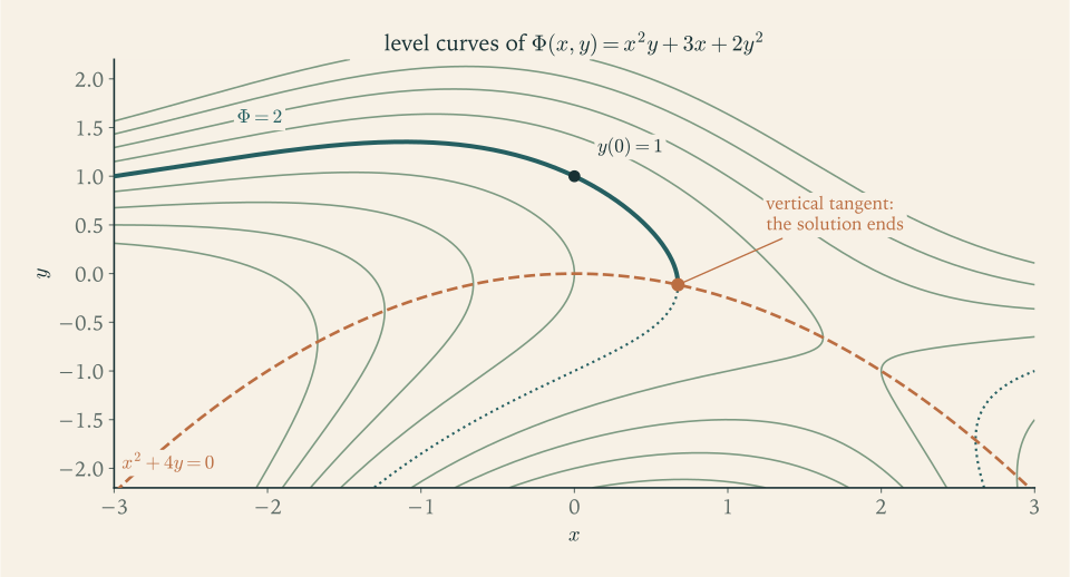
Level curves of the potential x squared y plus 3x plus 2 y squared, with the solution through the point (0,1) drawn as a thick arc that ends where it meets the dashed parabola x squared plus 4y equals zero; the rest of that level curve continues below as a dotted line. — **Figure 2.1.** A solution of an exact equation is an arc of a level curve of the potential, and it ends where the level curve becomes vertical. The dashed parabola is the set where N vanishes; beyond it the same level curve belongs to a different solution.

Figure 2.1 explains what the algebra reported. The level set \(\Phi=2\) is a perfectly good curve, but it is not the graph of one function of \(x\) : it doubles back at the dashed parabola. The solution of the initial value problem is the arc through \((0,1)\) up to the turning point. An implicit answer \(\Phi(x,y)=C\) is a correct description of the solution curves, but it does not by itself say which arc is the solution or where its interval ends.

When the test fails, the equation may become exact after multiplication by a suitable function, again called an integrating factor. Multiply by \(\mu(x)\) , a function of \(x\) alone. Exactness of \(\mu M\,dx+\mu N\,dy=0\) requires \(\mu M_y=\mu'N+\mu N_x\) , that is,

\[ \frac{\mu'}{\mu}=\frac{M_y-N_x}{N}. \]

The left side depends only on \(x\) . So an integrating factor \(\mu(x)\) exists precisely when the quotient \((M_y-N_x)/N\) is a function of \(x\) alone, and then \(\mu=\exp\int\frac{M_y-N_x}{N}\,dx\) . A linear equation \((p(x)y-q(x))\,dx+dy=0\) has \(M_y-N_x=p(x)\) and \(N=1\) , and the recipe returns \(\mu=e^{\int p}\) : the integrating factor of Section 2.2 is this one.

Example 2.6: Making an equation exact

Solve \((3xy+y^2)\,dx+(x^2+xy)\,dy=0\) for \(x>0\) .

Here \(M_y=3x+2y\) and \(N_x=2x+y\) , which differ, so the equation is not exact. The quotient

\[ \frac{M_y-N_x}{N}=\frac{x+y}{x(x+y)}=\frac1x \]

depends on \(x\) alone, so \(\mu=\exp(\ln x)=x\) . The multiplied equation is

\[ (3x^2y+xy^2)\,dx+(x^3+x^2y)\,dy=0, \]

with \(\partial_y(3x^2y+xy^2)=3x^2+2xy=\partial_x(x^3+x^2y)\) . Integrating the new \(M\) in \(x\) gives \(x^3y+\tfrac12x^2y^2+k(y)\) ; its \(y\) -derivative \(x^3+x^2y+k'(y)\) matches the new \(N\) with \(k'=0\) . The solutions are the level curves

\[ x^3y+\tfrac12x^2y^2=C . \]

For instance the solution with \(y(1)=1\) lies on the curve with \(C=3/2\) .

2.4 Changing the unknown

Some equations belong to none of the three classes as written but enter one of them after a change of variable.

Proposition 2.6 (Bernoulli equations). Let \(n\) be a real number other than \(0\) and \(1\) . If \(y\) is a positive solution of

\[ y'+p(t)\,y=q(t)\,y^{n}, \]

then \(v=y^{1-n}\) is a solution of the linear equation \(v'+(1-n)\,p(t)\,v=(1-n)\,q(t)\) , and conversely every positive solution \(v\) of the linear equation gives the solution \(y=v^{1/(1-n)}\) of the Bernoulli equation.

Proof. By the chain rule \(v'=(1-n)y^{-n}y'\) . Substituting \(y'=qy^{n}-py\) gives \(v'=(1-n)(q-py^{1-n})=(1-n)q-(1-n)pv\) . The steps are reversible when \(y>0\) .

When \(n\) is an integer the restriction to positive \(y\) can be relaxed to \(y\ne 0\) , and when \(n>0\) the constant function \(y=0\) is always an additional solution that the substitution does not see.

Example 2.7: A Bernoulli equation and its interval

Solve \(y'+y=ty^2\) , \(y(0)=1/2\) .

This is a Bernoulli equation with \(n=2\) , so \(v=y^{-1}\) . Then \(v'=-y'/y^2=-(ty^2-y)/y^2=-t+v\) , that is,

\[ v'-v=-t,\qquad v(0)=2 . \]

With integrating factor \(e^{-t}\) : \((e^{-t}v)'=-te^{-t}\) , and \(\int -te^{-t}\,dt=(t+1)e^{-t}+C\) , so \(v=t+1+Ce^{t}\) . The initial value gives \(C=1\) , and

\[ y(t)=\frac{1}{t+1+e^{t}} . \]

The denominator is increasing, positive at \(t=0\) , and vanishes at one point, \(t\approx-1.278\) . The solution therefore exists on \((-1.278,\infty)\) , tends to \(+\infty\) at the left end, and decays to \(0\) as \(t\to\infty\) .

A second useful substitution applies to equations in which the right-hand side depends only on the ratio \(y/t\) , such as \(y'=(t^2+y^2)/(ty)=t/y+y/t\) . Setting \(v=y/t\) , so that \(y=tv\) and \(y'=v+tv'\) , turns \(y'=F(y/t)\) into

\[ t\,v'=F(v)-v, \]

which is separable. For the equation just mentioned, \(F(v)=1/v+v\) , so \(tv'=1/v\) , \(v\,dv=dt/t\) , and \(\tfrac12v^2=\ln t+C\) for \(t>0\) . With \(y(1)=2\) the constant is \(C=2\) , and \(y=t\sqrt{2\ln t+4}\) , valid for \(t>e^{-2}\) .

2.5 Recognising the structure

The methods of this chapter apply to an equation only after it has been recognised, and several may apply at once. A workable order of questions is this.

Ask	Test	Then
Is it separable?	The right side of \(y'=f(t,y)\) factors as \(g(t)h(y)\)	List zeros of \(h\) ; integrate \(dy/h(y)=g(t)\,dt\)
Is it linear?	It can be written \(y'+p(t)y=q(t)\)	Multiply by \(e^{\int p}\) ; the interval is where \(p\) and \(q\) are continuous
Is it exact?	In the form \(M\,dx+N\,dy=0\) , \(M_y=N_x\)	Find a potential; solutions are level curves
Nearly exact?	\((M_y-N_x)/N\) depends on \(x\) only	Multiply by \(\exp\int(M_y-N_x)/N\,dx\)
Bernoulli?	\(y'+py=qy^n\)	Substitute \(v=y^{1-n}\)
Function of \(y/t\) ?	\(y'=F(y/t)\)	Substitute \(v=y/t\)

If every test fails, the equation probably has no elementary solution, and the right tools are the direction field, the phase line if the equation is autonomous, and numerical approximation. That is not a defeat. Most differential equations arising in practice are of this kind, and the qualitative questions, whether solutions exist, stay bounded, or approach an equilibrium, usually matter more than a formula.

Example 2.8: Classifying before computing

Consider again the three equations that opened the chapter, and a fourth.

The equation \(y'=ty\) is separable with \(h(y)=y\) , and also linear with \(p=-t\) , \(q=0\) . By either route the solutions are \(y=Ce^{t^2/2}\) , on \(\mathbb R\) ; the constant solution \(y=0\) is the case \(C=0\) , which the linear method finds automatically and the separable method finds only if the zero of \(h\) is listed.

The equation \(y'=t+y\) is linear: \(y'-y=t\) , \(\mu=e^{-t}\) , \((e^{-t}y)'=te^{-t}\) , so \(e^{-t}y=-(t+1)e^{-t}+C\) and \(y=-t-1+Ce^{t}\) . It is not separable and, written as \((t+y)\,dt-dy=0\) , not exact, since \(M_y=1\) and \(N_t=0\) .

The equation \(y'=t^2+y^2\) is not separable, not linear because of \(y^2\) , not Bernoulli because of the term \(t^2\) that carries no power of \(y\) , and not a function of \(y/t\) . It is a Riccati equation, and its solutions cannot be written with elementary functions. Its direction field (Exercise 1.7 treated a close relative) shows that every solution is increasing wherever \(t^2+y^2>0\) , and Chapter 3 will show that every solution blows up in finite time.

The equation \(y'=y-y^3\) is autonomous and therefore separable; it is also a Bernoulli equation with \(n=3\) . The fastest route to its long-term behaviour is neither: the phase line has equilibria \(-1\) , \(0\) , \(1\) with \(f'(\pm1)=-2\) and \(f'(0)=1\) , so every solution with \(y(0)>0\) tends to \(1\) and every solution with \(y(0)<0\) tends to \(-1\) . The explicit solution, \(y^2=1/(1+Ae^{-2t})\) , confirms this and adds the rate.

The lesson of the last case is general. A formula answers quantitative questions such as “when does \(y\) reach \(1/2\) ”; a phase line answers “where does \(y\) end up” faster and with less risk of algebraic error. Choosing the method includes choosing which question is being asked.

Exercises

Solve \(y'=2t\,(1+y^2)\) , \(y(0)=0\) , and state the interval of existence; then explain, using only the differential equation, why the solution must be an even function of \(t\) .

Answer

Separating, \(\arctan y=t^2+C\) with \(C=0\) , so \(y=\tan(t^2)\) on \(-\sqrt{\pi/2}<t<\sqrt{\pi/2}\) , about \(\lvert t\rvert<1.253\) . Evenness: if \(y\) is the solution then \(z(t)=y(-t)\) satisfies \(z'=-y'(-t)=2t\,(1+z^2)\) and \(z(0)=0\) , so \(z=y\) by the uniqueness in Theorem 2.2.
Solve \(y'=y^2-4\) with \(y(0)=0\) , listing the equilibrium solutions first, and express the answer without logarithms; state the limits of the solution as \(t\to\infty\) and as \(t\to-\infty\) .

Solution

The right-hand side \(h(y)=y^2-4\) vanishes at \(y=\pm2\) , so \(y=2\) and \(y=-2\) are equilibrium solutions. The initial value \(0\) lies in \(J=(-2,2)\) , where \(h<0\) , and by Theorem 2.2 the solution stays in \(J\) as long as the relation below can be solved.

Partial fractions give \(\dfrac{1}{y^2-4}=\dfrac14\Bigl(\dfrac{1}{y-2}-\dfrac{1}{y+2}\Bigr)\) , so on \(J\)

\[ \frac14\ln\frac{2-y}{2+y}=t+C . \]

At \(t=0\) , \(y=0\) gives \(C=0\) . Hence \((2-y)/(2+y)=e^{4t}\) , and solving for \(y\) ,

\[ y(t)=\frac{2\,(1-e^{4t})}{1+e^{4t}}=-2\tanh(2t). \]

The formula is defined for all \(t\) and stays in \((-2,2)\) , so the interval of existence is \(\mathbb R\) . As \(t\to\infty\) , \(y\to-2\) ; as \(t\to-\infty\) , \(y\to2\) . This matches the phase line: \(h<0\) between the equilibria, so the solution decreases from the unstable equilibrium \(2\) toward the stable equilibrium \(-2\) .
Solve \(y'-2ty=t\) , \(y(0)=1\) , by an integrating factor, and then again by separating variables, and confirm that the two answers agree.

Answer

Integrating factor \(e^{-t^2}\) : \((e^{-t^2}y)'=te^{-t^2}\) , so \(y=-\tfrac12+Ce^{t^2}\) and \(C=\tfrac32\) . Separable form: \(y'=t\,(1+2y)\) , so \(\tfrac12\ln(1+2y)=\tfrac12t^2+c\) , \(1+2y=3e^{t^2}\) . Both give \(y=\tfrac32e^{t^2}-\tfrac12\) .
Find all solutions of \(ty'+3y=6t^3\) on \((0,\infty)\) and identify the only one that stays bounded as \(t\to 0^{+}\) ; explain why Theorem 2.3 does not guarantee a solution through a prescribed value at \(t=0\) .

Solution

In normal form the equation is \(y'+\dfrac3t\,y=6t^2\) on \((0,\infty)\) . An integrating factor is \(\mu=\exp(3\ln t)=t^3\) , and

\[ (t^3y)'=6t^5,\qquad t^3y=t^6+C,\qquad y=t^3+\frac{C}{t^3}. \]

By Theorem 2.3 these are all the solutions on \((0,\infty)\) . As \(t\to0^{+}\) the term \(C/t^3\) is unbounded unless \(C=0\) , so the only solution that stays bounded is \(y=t^3\) .

Theorem 2.3 requires \(p\) and \(q\) to be continuous on an open interval containing the initial time. Here \(p(t)=3/t\) is not defined at \(t=0\) , so no interval containing \(0\) qualifies and the theorem is silent about data at \(t=0\) . In fact the original equation at \(t=0\) reads \(3y(0)=0\) , so only the value \(y(0)=0\) is possible there, and it is attained by exactly one of the solutions, \(y=t^3\) .
Test \((y\cos x+2xe^{y})\,dx+(\sin x+x^2e^{y}-1)\,dy=0\) for exactness, find a potential, and give the equation of the solution curve through the point \((0,2)\) .

Answer

\(M_y=\cos x+2xe^{y}=N_x\) , so the equation is exact. A potential is \(\Phi=y\sin x+x^2e^{y}-y\) . At \((0,2)\) , \(\Phi=-2\) , so the curve is \(y\sin x+x^2e^{y}-y=-2\) .
Show that \(M\,dx+N\,dy=0\) has an integrating factor depending on \(y\) alone exactly when \((N_x-M_y)/M\) is a function of \(y\) alone, and use this to solve \(y\,dx+(2x-ye^{y})\,dy=0\) for \(y>0\) .

Solution

Multiply by \(\mu(y)\) . The new equation \(\mu M\,dx+\mu N\,dy=0\) is exact when \((\mu M)_y=(\mu N)_x\) , that is, \(\mu'M+\mu M_y=\mu N_x\) , or

\[ \frac{\mu'}{\mu}=\frac{N_x-M_y}{M}. \]

The left side is a function of \(y\) alone. So a factor \(\mu(y)\) exists exactly when the right side is a function of \(y\) alone, and then \(\mu=\exp\int\frac{N_x-M_y}{M}\,dy\) .

For \(y\,dx+(2x-ye^{y})\,dy=0\) : \(M=y\) , \(N=2x-ye^{y}\) , \(M_y=1\) , \(N_x=2\) , and \((N_x-M_y)/M=1/y\) . Hence \(\mu=y\) , and the multiplied equation is

\[ y^2\,dx+(2xy-y^2e^{y})\,dy=0, \]

with both cross-derivatives equal to \(2y\) . Integrating \(y^2\) in \(x\) gives \(\Phi=xy^2+k(y)\) , and \(\Phi_y=2xy+k'(y)\) must equal \(2xy-y^2e^{y}\) , so \(k'=-y^2e^{y}\) and, integrating by parts twice, \(k=-(y^2-2y+2)e^{y}\) . The solutions are the level curves

\[ xy^2-(y^2-2y+2)e^{y}=C . \]

Here it is natural to solve for \(x\) as a function of \(y\) : \(x=\bigl(C+(y^2-2y+2)e^{y}\bigr)/y^2\) .
Solve the Bernoulli equation \(y'+y/t=y^2\) with \(y(1)=1\) and determine the interval of existence.

Answer

With \(v=1/y\) : \(v'-v/t=-1\) , \((v/t)'=-1/t\) , \(v=t\,(C-\ln t)\) , and \(v(1)=1\) gives \(C=1\) . So \(y=\dfrac{1}{t\,(1-\ln t)}\) on \(0<t<e\) ; it blows up at both ends.
Solve \(y'=(t+y)/(t-y)\) by the substitution \(v=y/t\) and show that in polar coordinates \(t=r\cos\theta\) , \(y=r\sin\theta\) the solution curves are the spirals \(r=Ae^{\theta}\) .

Solution

The right-hand side is a function of \(v=y/t\) : dividing numerator and denominator by \(t\) gives \(y'=(1+v)/(1-v)\) . With \(y=tv\) , \(y'=v+tv'\) , so

\[ tv'=\frac{1+v}{1-v}-v=\frac{1+v^2}{1-v},\qquad \frac{1-v}{1+v^2}\,dv=\frac{dt}{t}. \]

Integrating, for \(t>0\) ,

\[ \arctan v-\tfrac12\ln(1+v^2)=\ln t+C . \]

Now pass to polar coordinates with \(-\pi/2<\theta<\pi/2\) . Then \(v=y/t=\tan\theta\) , so \(\arctan v=\theta\) and \(1+v^2=1/\cos^2\theta\) , giving \(-\tfrac12\ln(1+v^2)=\ln\cos\theta\) . Also \(\ln t=\ln r+\ln\cos\theta\) . The relation becomes

\[ \theta+\ln\cos\theta=\ln r+\ln\cos\theta+C, \]

so \(\ln r=\theta-C\) and \(r=Ae^{\theta}\) with \(A=e^{-C}>0\) . The solution curves are logarithmic spirals. The same computation in the half-plane \(t<0\) gives the continuation of the same spirals. Each spiral crosses the line \(y=t\) , where the equation is undefined, with a vertical tangent, so a single solution \(y(t)\) is only an arc of a spiral between two such crossings.
For each equation name every method of this chapter that applies, without solving: (a) \(y'=e^{t-y}\) ; (b) \(ty'=y+t^3\) ; (c) \(2xy\,dx+(x^2+1)\,dy=0\) ; (d) \(y'=y-ty^3\) ; (e) \(y'=\sin(ty)\) .

Answer

(a) Separable: \(y'=e^{t}e^{-y}\) . (b) Linear: \(y'-y/t=t^2\) . (c) Exact, since \(M_y=2x=N_x\) ; also separable and linear, because \((x^2+1)y'=-2xy\) . (d) Bernoulli with \(n=3\) ; not separable. (e) None; use the direction field or numerics.
A student solves \(y'=y^2\) by separation, obtains \(y=-1/(t+C)\) , and concludes that the problem \(y(0)=0\) has no solution because no value of \(C\) gives \(y(0)=0\) . Identify the step at which a solution was lost and give the correct answer.

Solution

The equation is \(y'=g(t)h(y)\) with \(g=1\) and \(h(y)=y^2\) . The student divided by \(y^2\) to write \(dy/y^2=dt\) . That division is legitimate only where \(y\ne0\) , so everything derived afterwards describes only solutions that never take the value \(0\) . The zero of \(h\) at \(y=0\) gives the constant solution \(y(t)=0\) , by part (a) of Theorem 2.2, and it was lost at the moment of division.

The correct statement is that the solutions of \(y'=y^2\) are the functions \(y=-1/(t+C)\) , each on an interval not containing \(t=-C\) , together with the constant solution \(y=0\) . The initial value problem with \(y(0)=0\) has the solution \(y=0\) on \(\mathbb R\) . It is the only solution, because \(y^2\) is continuously differentiable and the uniqueness theorem of Chapter 3 applies. One can see the zero solution as the limit of the family as \(C\to\pm\infty\) , but it corresponds to no finite \(C\) .
A student solves \(2y'+6y=e^{-t}\) using the integrating factor \(e^{6t}\) and obtains \(y=\tfrac15e^{-t}+Ce^{-6t}\) . Show by substitution that this is wrong, locate the error, and find the correct general solution.

Answer

Substituting \(y=\tfrac15e^{-t}\) gives \(2y'+6y=\tfrac45e^{-t}\ne e^{-t}\) . The error is that the equation was not put in normal form: dividing by \(2\) gives \(y'+3y=\tfrac12e^{-t}\) , so \(\mu=e^{3t}\) , \((e^{3t}y)'=\tfrac12e^{2t}\) , and \(y=\tfrac14e^{-t}+Ce^{-3t}\) .
Let \(p\) and \(q\) be continuous on \(I\) . Prove that the difference of two solutions of \(y'+py=q\) on \(I\) is a solution of \(y'+py=0\) , and deduce that the graphs of two different solutions never meet.

Hint

Subtract the two equations. For the second part, the difference \(w\) solves \(w'+pw=0\) with the formula \(w=w(t_0)/\mu(t)\) ; if \(w\) vanishes at one point, what does the formula say everywhere?
Solve the variable-volume tank problem of Exercise 1.4, \(Q'+\dfrac{2Q}{100+t}=1.5\) with \(Q(0)=0\) , by an integrating factor, and so derive the formula that the earlier exercise only asked you to verify.

Solution

The equation is linear with \(p(t)=2/(100+t)\) , continuous for \(t>-100\) . An integrating factor is

\[ \mu=\exp\Bigl(\int\frac{2\,dt}{100+t}\Bigr)=\exp\bigl(2\ln(100+t)\bigr)=(100+t)^2 . \]

Multiplying the equation by \(\mu\) gives

\[ \bigl((100+t)^2Q\bigr)'=1.5\,(100+t)^2,\qquad (100+t)^2Q=0.5\,(100+t)^3+C . \]

The initial condition \(Q(0)=0\) gives \(0=0.5\times10^{6}+C\) , so \(C=-500000\) and

\[ Q(t)=0.5\,(100+t)-\frac{500000}{(100+t)^2}. \]

This is the formula of Exercise 1.4. The first term is what the salt mass would be if the tank were always at the inflow concentration \(0.5\ \mathrm{kg/L}\) ; the second term is the deficit left over from the initial fresh water, and it decays like the inverse square of the volume because each litre of outflow removes salt in proportion to the current concentration.
For the logistic equation \(y'=ry(1-y/K)\) with \(r,K>0\) and \(0<y(0)=y_0<K\) , derive \(y(t)=Ky_0/\bigl(y_0+(K-y_0)e^{-rt}\bigr)\) , and find the time at which the population is growing fastest when \(y_0<K/2\) .

Solution

The equilibria are \(0\) and \(K\) , and \(y_0\) lies between them, where the right-hand side is positive. Write the equation as \(y'=\dfrac rK\,y\,(K-y)\) . Partial fractions give \(\dfrac{K}{y(K-y)}=\dfrac1y+\dfrac1{K-y}\) , so on \((0,K)\)

\[ \ln\frac{y}{K-y}=rt+C,\qquad C=\ln\frac{y_0}{K-y_0}. \]

Exponentiating, \(\dfrac{y}{K-y}=\dfrac{y_0}{K-y_0}e^{rt}\) . Solving for \(y\) and multiplying numerator and denominator by \((K-y_0)e^{-rt}\) ,

\[ y(t)=\frac{Ky_0}{y_0+(K-y_0)e^{-rt}} . \]

The growth rate \(ry(1-y/K)\) is a downward parabola in \(y\) with its maximum at \(y=K/2\) . If \(y_0<K/2\) the increasing solution passes through \(K/2\) exactly once, when \(y/(K-y)=1\) , that is, when \(e^{rt}=(K-y_0)/y_0\) :

\[ t^{*}=\frac1r\ln\frac{K-y_0}{y_0}. \]

This is the inflection point of the S-shaped solution curve. If \(y_0\ge K/2\) the growth rate is already past its peak and decreases from the start.
Water drains from a tank so that its depth obeys Torricelli’s law \(h'=-k\sqrt h\) with \(k=0.2\ \mathrm{m^{1/2}/min}\) and \(h(0)=1\ \mathrm{m}\) . Solve for \(h(t)\) while \(h>0\) , find the time at which the tank is empty, and describe the solution after that time.

Answer

Separating, \(2\sqrt h=-kt+2\sqrt{h(0)}\) , so \(h(t)=(1-0.1\,t)^2\) metres for \(0\le t\le10\) . The tank is empty at \(t=10\ \mathrm{min}\) . For \(t\ge10\) the solution is \(h=0\) , the equilibrium; the formula \((1-0.1t)^2\) must not be continued past \(t=10\) , where it would rise again.
Show that every separable equation, written as \(g(t)\,dt-\dfrac{1}{h(y)}\,dy=0\) , is exact where \(h\ne 0\) , and identify its potential in the notation of Theorem 2.2.

Hint

Compute \(M_y\) and \(N_t\) for \(M=g(t)\) , \(N=-1/h(y)\) . A potential is built from the two antiderivatives \(G\) and \(H\) of Theorem 2.2.
The curves \(y=Cx^2\) all satisfy \(y'=2y/x\) . Curves that cross every member of this family at right angles satisfy \(y'=-x/(2y)\) . Solve that equation and describe the orthogonal curves geometrically.

Hint

The equation is separable: \(2y\,dy=-x\,dx\) . The solution curves are \(x^2+2y^2=C\) , ellipses centred at the origin whose horizontal semi-axis is \(\sqrt2\) times the vertical one.
Find the solution of \(y'+ky=\cos\omega t\) , with \(k>0\) and \(\omega>0\) , that is periodic, write it in the form \(A\cos(\omega t-\phi)\) , and show that \(A=1/\sqrt{k^2+\omega^2}\) and \(\tan\phi=\omega/k\) ; then say what happens to \(A\) and \(\phi\) as \(\omega\to\infty\) .

Solution

By Theorem 2.3 the general solution is a particular solution plus \(Ce^{-kt}\) . The exponential term is not periodic unless \(C=0\) , so there is exactly one periodic solution, and it can be found by trying \(y=a\cos\omega t+b\sin\omega t\) . Substituting,

\[ y'+ky=(ka+\omega b)\cos\omega t+(kb-\omega a)\sin\omega t, \]

which equals \(\cos\omega t\) when \(ka+\omega b=1\) and \(kb-\omega a=0\) . Solving, \(a=k/(k^2+\omega^2)\) and \(b=\omega/(k^2+\omega^2)\) :

\[ y=\frac{k\cos\omega t+\omega\sin\omega t}{k^2+\omega^2}. \]

To write this as \(A\cos(\omega t-\phi)=A\cos\phi\cos\omega t+A\sin\phi\sin\omega t\) we need \(A\cos\phi=a\) and \(A\sin\phi=b\) . Then \(A=\sqrt{a^2+b^2}=1/\sqrt{k^2+\omega^2}\) and \(\tan\phi=b/a=\omega/k\) , with \(0<\phi<\pi/2\) since \(a\) and \(b\) are positive.

As \(\omega\to\infty\) the amplitude \(A\) tends to \(0\) and the lag \(\phi\) tends to \(\pi/2\) : a first-order system cannot follow a rapidly oscillating input, and what little response there is trails the input by a quarter of a cycle. With \(k=2\) and \(\omega=1\) this reproduces Example 2.4 after multiplying by \(5\) : amplitude \(5/\sqrt5=\sqrt5\) and \(\tan\phi=1/2\) .