A cup of coffee at \(90^{\circ}\mathrm{C}\) is left on a desk in a room at \(20^{\circ}\mathrm{C}\) . Ten minutes later it has cooled to \(60^{\circ}\mathrm{C}\) . When will it reach a drinkable \(40^{\circ}\mathrm{C}\) ?
Linear interpolation gives a wrong answer. The coffee lost \(30\) degrees in the first ten minutes, but it will not lose \(30\) more in the next ten, because it cools more slowly as it approaches room temperature. What stays the same from minute to minute is not the rate of cooling but the rule for the rate: at each instant the temperature falls at a rate proportional to its excess over the surroundings. That rule is a differential equation. This chapter explains what such an equation asserts, what it means to solve one, how to build one from a physical law, and how to read the behaviour of solutions directly from the equation, by picture and by arithmetic, before any solution formula is available.
1.1 Equations, solutions, and intervals
Definition 1.1 (ordinary differential equation, order). An ordinary differential equation for an unknown function \(y\) of one variable \(t\) is an equation relating \(t\) , \(y(t)\) , and finitely many derivatives of \(y\) at \(t\) . Its order is the order of the highest derivative that appears. A first-order equation in normal form is
where \(f\) is a given function of two variables.
The equation \(y'=-2y\) is first order. The pendulum equation \(\theta''+\sin\theta=0\) is second order. The word ordinary separates these from partial differential equations, in which the unknown depends on several variables.
Definition 1.2 (solution on an interval). A solution of \(y'=f(t,y)\) on an open interval \(I\) is a function \(y\) that is differentiable at every point of \(I\) and satisfies \(y'(t)=f(t,y(t))\) for every \(t\in I\) ; in particular \((t,y(t))\) must lie in the domain of \(f\) for every \(t\in I\) . A solution of an equation of order \(n\) is defined in the same way with \(n\) derivatives.
Two features of this definition are easy to overlook and will matter throughout the book. A solution is a function together with an interval; the same formula on a different interval is a different solution, or no solution at all. And the equation must hold at every point of the interval, not at most points.
Definition 1.3 (initial value problem). An initial value problem for a first-order equation consists of the equation and one condition at a point:
A solution is a solution of the equation on an open interval \(I\) containing \(t_0\) that takes the value \(y_0\) at \(t_0\) . For an equation of order \(n\) the initial data are the values \(y(t_0),y'(t_0),\dots,y^{(n-1)}(t_0)\) .
A differential equation alone usually has infinitely many solutions. For \(y'=-2y\) every function \(y=Ce^{-2t}\) is a solution on \(\mathbb R\) , one for each real constant \(C\) . Such a formula containing an arbitrary constant is called a general solution when it captures every solution, and that claim always needs an argument. Here is one. If \(y\) is any solution of \(y'=-2y\) on an interval, then
so \(e^{2t}y(t)\) is a constant \(C\) on that interval and \(y=Ce^{-2t}\) . The initial condition then picks one member of the family: \(y(0)=3\) forces \(C=3\) .
Example 1.1: Checking a solution and finding its interval
Consider the initial value problem \(y'=y^2\) , \(y(0)=1\) , and the candidate \(y(t)=1/(1-t)\) .
The equation. Differentiating, \(y'(t)=1/(1-t)^2\) , and \(y(t)^2=1/(1-t)^2\) , so \(y'=y^2\) wherever the formula makes sense, that is, for \(t\ne 1\) .
The datum. \(y(0)=1/(1-0)=1\) .
The interval. The formula is defined on two separate intervals, \((-\infty,1)\) and \((1,\infty)\) . A solution of the initial value problem must live on an interval containing \(t_0=0\) , so the solution is \(y(t)=1/(1-t)\) on \((-\infty,1)\) , and it cannot be extended further to the right as a solution because \(y(t)\to+\infty\) as \(t\to 1\) from the left.
The branch of the same formula on \((1,\infty)\) is also a solution of the differential equation, but it is negative, it has nothing to do with the initial condition \(y(0)=1\) , and it would be a serious error to use it to “predict” \(y(2)=-1\) . A quantity that starts positive and obeys \(y'=y^2\) only increases; it becomes infinite at time \(1\) and the model says nothing after that. Chapter 3 studies this finite-time blow-up systematically.
A function can also fail to be a solution at a single point. The function \(y(t)=\lvert t\rvert\) satisfies \((y')^2=1\) at every \(t\ne 0\) , but it is not differentiable at \(0\) , so it is not a solution of \((y')^2=1\) on any interval containing \(0\) .
Definition 1.4 (linear and autonomous equations). A first-order equation is linear if it can be written \(y'+p(t)y=q(t)\) ; an equation of order \(n\) is linear if it has the form \(a_n(t)y^{(n)}+\dots+a_1(t)y'+a_0(t)y=g(t)\) . It is homogeneous if the right-hand side is zero. An equation that is not linear is nonlinear. A first-order equation is autonomous if the right-hand side does not depend on \(t\) : \(y'=f(y)\) .
Linearity refers to how the unknown \(y\) and its derivatives enter, not to how \(t\) enters: \(y'+t^2y=\sin t\) is linear, while \(y'=y^2\) and \(y'=\sin y\) are not. Autonomous equations describe systems whose law does not change with time; the cooling law is one, because the rule relating rate to temperature is the same at noon and at midnight.
An equation of higher order can always be rewritten as a system of first-order equations. For \(y''+3y'+2y=\cos t\) , put \(x_1=y\) and \(x_2=y'\) ; then
The two initial data \(y(t_0)\) and \(y'(t_0)\) become the single initial vector \((x_1(t_0),x_2(t_0))\) . This is why an equation of order \(n\) needs \(n\) initial conditions, and it is the form in which Chapter 7 treats all linear equations at once.
1.2 From a rate law to an equation
Building a model is a matter of saying, in symbols and with units, what changes the quantity of interest. Three steps recur. Name the unknown function and its units. Write the rate of change as a sum of contributions, each justified by a stated assumption. Check that every term has the units of the unknown per unit time.
Example 1.2: The cooling coffee
Let \(T(t)\) be the temperature of the coffee in degrees Celsius at time \(t\) in minutes. Newton’s law of cooling assumes that the rate of change of \(T\) is proportional to the difference between \(T\) and the ambient temperature \(A\) :
with \(k>0\) a constant with units of \(1/\mathrm{min}\) , so that both sides have units of degrees per minute. The sign is chosen so that an object warmer than its surroundings cools.
The substitution \(u=T-A\) turns the equation into \(u'=-ku\) , whose solutions are \(u=Ce^{-kt}\) by the argument given for \(y'=-2y\) . Hence
With \(A=20\) and \(T_0=90\) this is \(T(t)=20+70e^{-kt}\) . The measurement \(T(10)=60\) determines the constant: \(40=70e^{-10k}\) , so
The coffee reaches \(40^{\circ}\mathrm{C}\) when \(20=70e^{-kt}\) , that is, at
The second fall of twenty degrees takes about \(12.4\) minutes although the first thirty took only \(10\) . Two checks: the formula gives \(T(0)=90\) , and \(T(t)\to 20\) as \(t\to\infty\) , the room temperature, which no cooling object can pass.
The model has a boundary of validity. It assumes the room is so large that the coffee does not warm it, that the cup has one temperature throughout, and that evaporation is negligible. Each assumption can be questioned; the equation is what the assumptions imply, no more.
Example 1.3: Salt in a stirred tank
A tank holds \(100\ \mathrm{L}\) of water in which \(10\ \mathrm{kg}\) of salt is dissolved. Brine containing \(0.2\ \mathrm{kg/L}\) flows in at \(3\ \mathrm{L/min}\) , the tank is kept well stirred, and mixture flows out at \(3\ \mathrm{L/min}\) . Let \(Q(t)\) be the mass of salt in kilograms after \(t\) minutes.
Salt enters at \(0.2\times 3=0.6\ \mathrm{kg/min}\) . The volume stays at \(100\ \mathrm{L}\) because inflow equals outflow, so the concentration in the tank, and therefore in the outflow, is \(Q/100\ \mathrm{kg/L}\) , and salt leaves at \(3Q/100\ \mathrm{kg/min}\) . The balance rate of change equals rate in minus rate out reads
Writing the equation as \(Q'=-0.03\,(Q-20)\) shows it is the cooling equation in disguise, with “ambient” value \(20\) . Therefore
The salt mass rises from \(10\ \mathrm{kg}\) toward \(20\ \mathrm{kg}\) , which is the mass at which the tank’s concentration equals the inflow concentration \(0.2\ \mathrm{kg/L}\) . It reaches \(15\ \mathrm{kg}\) when \(e^{-0.03t}=1/2\) , at \(t=\ln 2/0.03\approx 23.1\ \mathrm{min}\) .
The “well stirred” assumption is what makes the outflow concentration equal to \(Q/V\) ; without it the tank would need a partial differential equation. The constant-volume assumption is what makes the coefficient \(0.03\) constant; Exercise 4 removes it.
Common mistake. Checking that a formula satisfies the differential equation and stopping there. A complete verification has three lines: the equation, each initial datum, and the interval. In Example 1.1 the formula \(1/(1-t)\) satisfies the equation at \(t=2\) , yet \(y(2)=-1\) is not a value of the solution of the initial value problem, whose interval ends at \(t=1\) . Likewise \(Q=20+Ce^{-0.03t}\) satisfies the tank equation for every \(C\) , but only \(C=-10\) describes this tank.
1.3 Direction fields
The equation \(y'=f(t,y)\) has a direct geometric meaning. At each point \((t,y)\) of the plane it prescribes a number \(f(t,y)\) , and a solution passing through that point must have exactly that slope there. Drawing a short segment of slope \(f(t,y)\) at each point of a grid gives the direction field of the equation. A solution is a curve that is tangent to the field at every one of its points. The field can be drawn without solving anything, and it often shows the fate of every solution at a glance.
An isocline is a curve along which the slope is constant: the set where \(f(t,y)=c\) . The isocline for \(c=0\) is especially useful, since solutions cross it horizontally and it separates the region where solutions rise from the region where they fall.
Example 1.4: Reading the field of a linear equation
For \(y'=t-y\) the isoclines are the lines \(y=t-c\) , each a line of slope \(1\) . On the line \(y=t\) the field is horizontal. Above that line \(t-y<0\) and solutions fall; below it they rise.
One isocline is special. On \(y=t-1\) the prescribed slope is \(c=1\) , which equals the slope of the line itself. So the line \(y=t-1\) is tangent to the field at each of its points: it is a solution. The check is immediate, since \(y=t-1\) gives \(y'=1\) and \(t-y=1\) .
To see what other solutions do relative to this one, set \(w=y-(t-1)\) , the vertical distance above the line. Then \(w'=y'-1=t-y-1=-w\) , so \(w=Ce^{-t}\) and
Every solution approaches the line \(y=t-1\) as \(t\to\infty\) , from above if \(C>0\) and from below if \(C<0\) , and the distance to it shrinks by the factor \(e^{-1}\approx 0.37\) per unit time. A solution with \(C>0\) falls until it meets the line \(y=t\) , turns there, and then rises. Solving \(t-1+Ce^{-t}=t\) gives the turning time \(t=\ln C\) . For the solution through \((0,1)\) we have \(C=2\) , and the minimum is at \(t=\ln 2\approx 0.693\) with value \(y=\ln 2\approx 0.693\) .
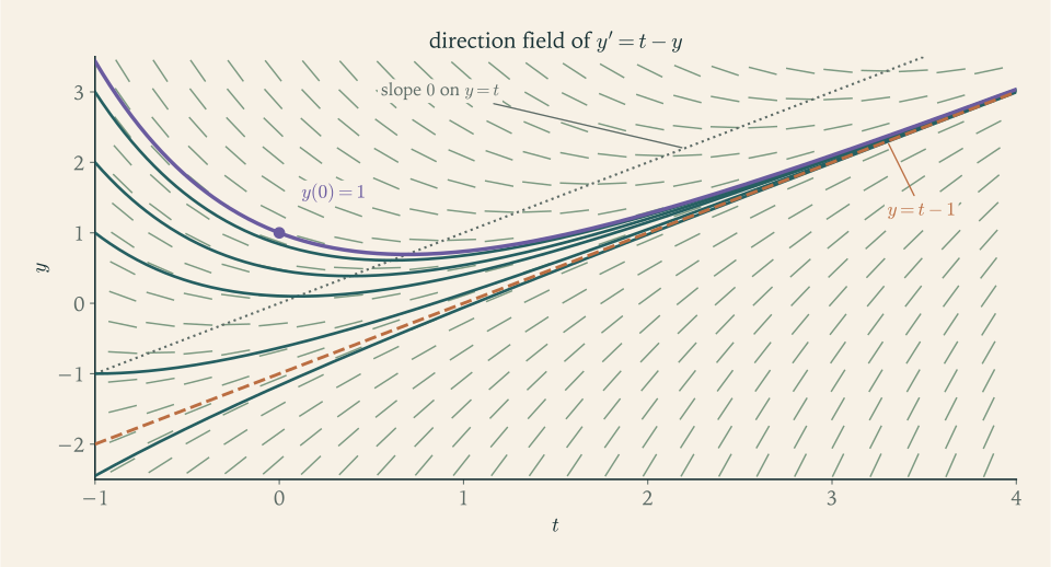
Figure 1.1 shows more than the formula does at first reading: solutions never cross one another, they are funnelled together as \(t\) increases and fan apart as \(t\) decreases, and the turning points all lie on one line. The non-crossing is not an accident of this example. It is the uniqueness theorem of Chapter 3 seen in a picture: two solution curves through a common point would be two solutions of one initial value problem.
1.4 Autonomous equations and the phase line
For an autonomous equation \(y'=f(y)\) the direction field does not depend on \(t\) : every horizontal line carries one slope. All the information is in the sign of \(f\) , and it can be recorded on a single vertical axis.
Definition 1.5 (equilibrium and phase line). An equilibrium of \(y'=f(y)\) is a number \(c\) with \(f(c)=0\) ; the constant function \(y(t)=c\) is then a solution. The phase line is the \(y\) -axis marked with the equilibria and, on each interval between them, an arrow pointing up where \(f>0\) and down where \(f<0\) . An equilibrium is called stable if the arrows on both sides point toward it, unstable if both point away, and semistable if one points toward it and one away.
The arrows describe what solutions do, and the next result makes that precise. It relies on uniqueness of solutions, which holds whenever \(f\) is continuously differentiable; that is Theorem 3.5, and it is used here in advance.
Proposition 1.6 (solutions of an autonomous equation are monotone). Let \(f\) be continuously differentiable on \(\mathbb R\) and let \(y\) be a solution of \(y'=f(y)\) on an interval \(I\) . If \(y\) takes an equilibrium value at one time, then \(y\) is constant. Otherwise \(y\) is strictly increasing or strictly decreasing on \(I\) and never takes an equilibrium value. If moreover \(I\) contains \([t_0,\infty)\) and \(y\) is bounded there, then \(y(t)\) converges as \(t\to\infty\) , and its limit is an equilibrium.
Proof. Suppose \(y(t_1)=c\) with \(f(c)=0\) . The constant function \(c\) and the function \(y\) both solve the initial value problem with datum \(c\) at time \(t_1\) , so by uniqueness they agree on \(I\) .
Otherwise \(f(y(t))\ne 0\) for every \(t\in I\) . The function \(t\mapsto f(y(t))\) is continuous on the interval \(I\) and never zero, so by the intermediate value theorem it has one sign throughout. Since \(y'=f(y)\) , the derivative of \(y\) has one sign, and \(y\) is strictly monotone.
For the last claim, a bounded monotone function has a limit \(L\) as \(t\to\infty\) . By continuity of \(f\) , \(y'(t)=f(y(t))\to f(L)\) . If \(f(L)>0\) , there is a time \(T\) after which \(y'(t)\ge f(L)/2\) , and then \(y(t)\ge y(T)+(t-T)f(L)/2\) , which is unbounded, a contradiction. The case \(f(L)<0\) is symmetric. Hence \(f(L)=0\) .
So a solution of an autonomous equation, started between two consecutive equilibria, stays between them forever and slides monotonically toward the one the arrow points to. There is also a derivative test. If \(f(c)=0\) and \(f'(c)<0\) , then \(f\) changes sign from positive to negative at \(c\) and the equilibrium is stable; if \(f'(c)>0\) it is unstable; if \(f'(c)=0\) the test says nothing and one must look at the signs directly.
Example 1.5: A fishery with a constant catch
A fish population \(y\) , measured in thousands of tonnes, grows logistically with carrying capacity \(4\) and is fished at the constant rate \(3/4\) per year:
Multiplying out, \(y'=-\tfrac14(y^2-4y+3)=-\tfrac14(y-1)(y-3)\) . The equilibria are \(y=1\) and \(y=3\) . The right-hand side is negative for \(y<1\) , positive for \(1<y<3\) , and negative for \(y>3\) . So \(y=3\) is stable and \(y=1\) is unstable; the derivative test agrees, because \(f'(y)=1-y/2\) gives \(f'(1)=1/2\) and \(f'(3)=-1/2\) .
By Proposition 1.6 a population that starts above \(1\) tends to \(3\) , whether it starts at \(1.1\) or at \(40\) . A population that starts below \(1\) decreases, and since there is no equilibrium below \(1\) for it to approach, it cannot stay bounded below: it reaches \(0\) in finite time, where the model stops making sense and the fishery has collapsed. The unstable equilibrium \(y=1\) is a threshold, not a state one would ever observe.
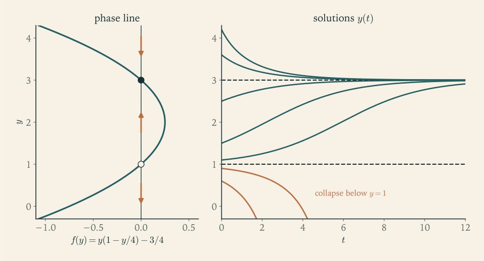
The catch rate matters. The growth term \(y(1-y/4)\) has maximum value \(1\) , attained at \(y=2\) . With catch rate \(h\) in place of \(3/4\) , the equilibria are the roots of \(y^2-4y+4h=0\) , namely \(y=2\pm 2\sqrt{1-h}\) . For \(h<1\) there are two; at \(h=1\) they merge into the single semistable equilibrium \(y=2\) ; for \(h>1\) there are none, the right-hand side is negative everywhere, and every population collapses. A qualitative change of this kind in the set of equilibria as a parameter passes a critical value is called a bifurcation.
1.5 Stepping along the field: Euler’s method
The direction field suggests a way to approximate a solution: start at the initial point, walk a short distance in the direction the field prescribes, look at the field again, and repeat.
Definition 1.7 (Euler’s method). For the initial value problem \(y'=f(t,y)\) , \(y(t_0)=y_0\) , and a step size \(h>0\) , Euler’s method produces the points
and takes \(y_n\) as an approximation to \(y(t_n)\) .
Each step replaces the solution by its tangent line at the current point. The tangent line is a good approximation only briefly, and the errors of successive steps accumulate, so the method is a rough one. Its value in this book is conceptual: it shows that an initial value problem contains, in principle, all the information needed to compute its solution, and it gives a number to compare with when a formula is in doubt.
Example 1.6: Euler’s method against an exact solution
Take \(y'=t-y\) , \(y(0)=1\) . By Example 1.4 the exact solution is \(y(t)=t-1+2e^{-t}\) .
With \(h=0.1\) , the first step uses the slope \(f(0,1)=-1\) :
The second step uses the slope at the new point, \(f(0.1,0.9)=-0.8\) :
The exact values are \(y(0.1)\approx 0.9097\) and \(y(0.2)\approx 0.8375\) , so the errors after one and two steps are about \(0.0097\) and \(0.0175\) .
Halving the step to \(h=0.05\) and taking two steps to reach \(t=0.1\) gives \(y_1=1+0.05\,(0-1)=0.95\) and \(y_2=0.95+0.05\,(0.05-0.95)=0.905\) , with error about \(0.0047\) , roughly half the error of the single step of size \(0.1\) .
The same pattern holds at a fixed later time. Carrying the computation to \(t=1\) , where the exact value is \(2/e\approx 0.73576\) , gives the following.
| Step size \(h\) | Steps | Euler value at \(t=1\) | Error |
|---|---|---|---|
| \(0.1\) | \(10\) | \(0.69736\) | \(0.03840\) |
| \(0.05\) | \(20\) | \(0.71697\) | \(0.01879\) |
| \(0.025\) | \(40\) | \(0.72646\) | \(0.00929\) |
Each halving of \(h\)
roughly halves the error. Euler’s method is said to be of first order: under smoothness assumptions on \(f\)
, the error at a fixed time is bounded by a constant times \(h\)
. The proof, and methods of higher order, belong to Numerical Analysis (math.numerical-analysis.ode-initial-value).
Common mistake. Trusting a numerical solution because it looks smooth. Apply Euler’s method with \(h=0.3\) to \(y'=-10y\) , \(y(0)=1\) , whose solution \(e^{-10t}\) decays rapidly to zero. Each step multiplies the current value by \(1-10h=-2\) , so the computed values are \(1,-2,4,-8,\dots\) : they alternate in sign and grow. Nothing in the differential equation oscillates or grows; the behaviour is produced entirely by the step size. Before believing a computed solution, repeat the computation with half the step and compare, and check that the result respects what the phase line or direction field predicts.
The tools of this chapter, verification, direction fields, phase lines, and stepping, apply to every first-order equation. What they do not provide is formulas. The next chapter supplies formulas for the classes of equations that have them, and Chapter 3 returns to the questions that this chapter used without proof: whether a solution exists through each point, and whether it is the only one.
Exercises
-
Show that \(y=t-1+e^{-t}\) is a solution of \(y'=t-y\) on \(\mathbb R\) and state the initial condition it satisfies at \(t=0\) ; then find the member of the family \(y=t-1+Ce^{-t}\) that satisfies \(y(1)=2\) .
Answer
\(y'=1-e^{-t}\) and \(t-y=1-e^{-t}\) , so the equation holds for all \(t\) ; \(y(0)=0\) . For \(y(1)=2\) : \(1-1+Ce^{-1}=2\) gives \(C=2e\) , so \(y=t-1+2e^{1-t}\) .
-
Give the order of each equation and say whether it is linear, and for the first-order ones whether it is autonomous: (a) \(y'=ty^2\) ; (b) \(y''+ty=\sin t\) ; (c) \(y'=y(1-y)\) ; (d) \(y'''+yy'=0\) ; (e) \(t^2y''+ty'+y=0\) .
Answer
(a) First order, nonlinear, not autonomous. (b) Second order, linear. (c) First order, nonlinear, autonomous. (d) Third order, nonlinear because of the product \(yy'\) . (e) Second order, linear and homogeneous; the coefficients depend on \(t\) , which does not affect linearity.
-
A thermometer reading \(5^{\circ}\mathrm{C}\) is carried into a room at \(22^{\circ}\mathrm{C}\) , and one minute later it reads \(12^{\circ}\mathrm{C}\) . Write the initial value problem given by Newton’s law with units for every quantity, solve it, and find when the reading is \(20^{\circ}\mathrm{C}\) .
Solution
Let \(T(t)\) be the reading in degrees Celsius after \(t\) minutes in the room. Newton’s law gives
\[ T'=-k\,(T-22),\qquad T(0)=5, \]with \(k\) in \(\mathrm{min}^{-1}\) , so both sides are in degrees per minute. Here the thermometer is colder than the room, \(T-22<0\) , and the equation makes \(T'>0\) , as it should. The difference \(u=T-22\) satisfies \(u'=-ku\) , so \(u=u(0)e^{-kt}=-17e^{-kt}\) and
\[ T(t)=22-17e^{-kt}. \]The reading \(T(1)=12\) gives \(17e^{-k}=10\) , so \(k=\ln(17/10)\approx 0.531\ \mathrm{min}^{-1}\) . The reading is \(20\) when \(17e^{-kt}=2\) , that is, at
\[ t=\frac{\ln(17/2)}{\ln(17/10)}\approx 4.03\ \mathrm{min}. \]Check: \(T(0)=22-17=5\) , and \(T\to 22\) as \(t\to\infty\) . The thermometer needs about four minutes to come within two degrees of the room, although it covered the first seven degrees in one minute.
-
A \(200\ \mathrm{L}\) tank initially holds \(100\ \mathrm{L}\) of pure water. Brine with \(0.5\ \mathrm{kg/L}\) of salt enters at \(3\ \mathrm{L/min}\) and the stirred mixture leaves at \(2\ \mathrm{L/min}\) . Derive the initial value problem for the salt mass \(Q(t)\) , state the time interval on which the model is valid, verify that \(Q(t)=0.5\,(100+t)-500000/(100+t)^2\) solves it, and find the salt mass when the tank is full.
Solution
The volume is no longer constant: it grows at \(3-2=1\ \mathrm{L/min}\) , so \(V(t)=100+t\) litres. Salt enters at \(0.5\times 3=1.5\ \mathrm{kg/min}\) . The concentration in the tank is \(Q/(100+t)\ \mathrm{kg/L}\) and mixture leaves at \(2\ \mathrm{L/min}\) , so salt leaves at \(2Q/(100+t)\ \mathrm{kg/min}\) . Hence
\[ Q'=1.5-\frac{2Q}{100+t},\qquad Q(0)=0 . \]The tank is full when \(100+t=200\) , so the model is valid for \(0\le t\le 100\) ; after that the tank overflows and the outflow rate changes.
To verify the formula, write \(s=100+t\) , so \(Q=0.5s-500000\,s^{-2}\) and \(Q'=0.5+1000000\,s^{-3}\) . On the other side,
\[ 1.5-\frac{2Q}{s}=1.5-1+1000000\,s^{-3}=0.5+1000000\,s^{-3}. \]The two agree. At \(t=0\) , \(Q=50-500000/10000=0\) . So the formula solves the initial value problem on \([0,100]\) . When the tank is full, \(s=200\) and
\[ Q(100)=100-\frac{500000}{40000}=87.5\ \mathrm{kg}. \]The concentration at that moment is \(87.5/200\approx 0.44\ \mathrm{kg/L}\) , still below the inflow concentration \(0.5\) , as it must be since the tank started with fresh water.
-
Let \(y\) be a solution of the autonomous equation \(y'=f(y)\) on an interval \((a,b)\) and let \(c\) be a real number. Prove that \(z(t)=y(t+c)\) is a solution on \((a-c,b-c)\) , and explain what this says about the direction field.
Solution
For \(t\in(a-c,b-c)\) the number \(t+c\) lies in \((a,b)\) , so \(z(t)=y(t+c)\) is defined. By the chain rule \(z\) is differentiable and
\[ z'(t)=y'(t+c)\cdot 1=f\bigl(y(t+c)\bigr)=f\bigl(z(t)\bigr). \]The second equality is the differential equation for \(y\) evaluated at the time \(t+c\) , and it is here that autonomy is used: the right-hand side \(f\) is the same function at time \(t+c\) as at time \(t\) . For a non-autonomous equation the same computation gives \(z'(t)=f(t+c,z(t))\) , which is a different equation.
Geometrically, the direction field of an autonomous equation has the same slope all along each horizontal line, so sliding the whole picture left or right maps the field onto itself, and therefore maps solution curves onto solution curves. Every solution through the level \(y_0\) is a horizontal translate of one of them.
-
Draw the phase line of \(y'=y^2(1-y)\) , classify each equilibrium as stable, unstable, or semistable, and state the limit as \(t\to\infty\) of the solutions with \(y(0)=-1\) , \(y(0)=1/2\) , and \(y(0)=2\) .
Answer
Equilibria \(0\) and \(1\) . The right-hand side is positive for \(y<0\) and for \(0<y<1\) , and negative for \(y>1\) . So \(0\) is semistable (approached from below, left from above) and \(1\) is stable. Limits: \(y(0)=-1\) gives \(y\to 0\) ; \(y(0)=1/2\) gives \(y\to 1\) ; \(y(0)=2\) gives \(y\to 1\) .
-
For \(y'=t^2+y^2-1\) describe the isoclines, find the region of the plane in which solutions are decreasing, and explain why every solution that enters the region \(t>1\) is increasing from then on.
Hint
The isocline of slope \(c\) is the circle \(t^2+y^2=1+c\) , which exists for \(c>-1\) . Solutions decrease exactly where \(t^2+y^2<1\) . For the last part, compare \(t^2\) with \(1\) .
-
A student writes: “The solution of \(y'=y^2\) , \(y(0)=1\) is \(y=1/(1-t)\) , so \(y(2)=-1\) .” Explain precisely which part of the definition of a solution of an initial value problem the student has ignored, and say what the model predicts instead.
Solution
A solution of an initial value problem is a differentiable function on an open interval containing the initial time \(t_0=0\) and satisfying the equation at every point of that interval. The formula \(1/(1-t)\) is not defined at \(t=1\) , so no interval containing both \(0\) and \(2\) can serve as its domain. The solution of the initial value problem is \(1/(1-t)\) on \((-\infty,1)\) only. The value \(-1\) at \(t=2\) belongs to the other branch of the formula, which is a solution of the differential equation on \((1,\infty)\) but is unrelated to the datum \(y(0)=1\) .
What the model predicts is that \(y\) increases without bound as \(t\to 1\) from the left: since \(y'=y^2>0\) the solution is increasing, so it can never become negative after starting at \(1\) . The quantity becomes infinite at \(t=1\) , and for \(t\ge 1\) the model makes no prediction.
-
Apply Euler’s method with \(h=0.25\) to \(y'=y\) , \(y(0)=1\) on \([0,1]\) and compare the result with \(e\) . Then show that with step \(h=1/n\) the method gives \((1+1/n)^n\) at \(t=1\) , and say what happens as \(n\to\infty\) .
Solution
Here \(f(t,y)=y\) , so each Euler step is \(y_{n+1}=y_n+hy_n=(1+h)y_n\) . With \(h=0.25\) four steps reach \(t=1\) :
\[ y_1=1.25,\quad y_2=1.5625,\quad y_3=1.953125,\quad y_4=2.44140625 . \]The exact value is \(e\approx 2.71828\) , so the error is about \(0.277\) , roughly ten percent. The approximation is low because the solution is convex: each tangent line lies below the curve.
In general, with \(h=1/n\) the recursion gives \(y_k=(1+1/n)^k\) , and \(t=1\) is reached after \(n\) steps with value \((1+1/n)^n\) . As \(n\to\infty\) this tends to \(e\) , which is one of the standard definitions of \(e\) . So for this equation the convergence of Euler’s method as the step shrinks is exactly the classical limit \(\lim_{n\to\infty}(1+1/n)^n=e\) .
-
For \(y'=-10y\) , \(y(0)=1\) , show that Euler’s method with step \(h\) gives \(y_n=(1-10h)^n\) . Find all step sizes for which the computed values tend to \(0\) , and all step sizes for which they tend to \(0\) without changing sign.
Solution
With \(f(t,y)=-10y\) , a step is \(y_{n+1}=y_n-10hy_n=(1-10h)y_n\) , and \(y_0=1\) gives \(y_n=(1-10h)^n\) .
The powers of a number \(r\) tend to \(0\) exactly when \(\lvert r\rvert<1\) . With \(r=1-10h\) and \(h>0\) , the condition \(-1<1-10h<1\) is \(0<h<0.2\) . So the computed values tend to \(0\) for \(0<h<0.2\) . At \(h=0.2\) they are \(1,-1,1,\dots\) and for \(h>0.2\) they grow in size while alternating in sign.
The values keep one sign when \(r\ge 0\) , that is, when \(h\le 0.1\) . For \(0<h<0.1\) they are positive and decrease to \(0\) as the true solution does; at \(h=0.1\) the method jumps to \(0\) in one step and stays there. For \(0.1<h<0.2\) the values tend to \(0\) but alternate in sign, which the true solution \(e^{-10t}\) never does. The lesson is that a step can be small enough for convergence and still too large to reproduce the qualitative behaviour.
-
In the fishery model replace the catch rate \(3/4\) by a parameter \(h\ge 0\) . Find the equilibria as functions of \(h\) , sketch them against \(h\) in the \((h,y)\) plane, and describe the fate of a population starting at \(y=2\) when \(h=0.9\) , \(h=1\) , and \(h=1.1\) .
Solution
The equilibria solve \(y(1-y/4)-h=0\) , that is, \(y^2-4y+4h=0\) , so
\[ y=2\pm 2\sqrt{1-h}\qquad(0\le h\le 1). \]In the \((h,y)\) plane this is the parabola \(h=1-(y-2)^2/4\) opening to the left with vertex at \((1,2)\) . The upper branch is the stable equilibrium and the lower branch the unstable one, since the right-hand side \(-\tfrac14(y-2)^2+(1-h)\) is positive between the roots and negative outside.
For \(h=0.9\) the equilibria are \(2\pm 2\sqrt{0.1}\) , about \(1.37\) and \(2.63\) . The start \(y=2\) lies between them, so the population increases to about \(2.63\) . For \(h=1\) the only equilibrium is \(y=2\) , and a population starting exactly there stays there; any population starting below \(2\) collapses, so this state is not robust. For \(h=1.1\) the right-hand side is \(-\tfrac14(y-2)^2-0.1\le -0.1\) , so the population decreases at a rate of at least \(0.1\) and reaches \(0\) in at most \(20\) years; integrating \(dt=-4\,dy/((y-2)^2+0.4)\) from \(y=2\) to \(y=0\) gives the exact collapse time \((4/\sqrt{0.4})\arctan(2/\sqrt{0.4})\approx 8.0\) years.
-
A bacterial culture grows at a rate proportional to its size and doubles every \(3\) hours. Write the initial value problem for the size \(N(t)\) with initial size \(N_0\) , find the constant of proportionality with its units, and find how long the culture takes to grow tenfold.
Answer
\(N'=kN\) , \(N(0)=N_0\) , so \(N=N_0e^{kt}\) . Doubling in \(3\) hours gives \(k=\ln 2/3\approx 0.231\ \mathrm{h}^{-1}\) . Tenfold growth takes \(\ln 10/k=3\ln 10/\ln 2\approx 9.97\) hours.
-
Rewrite \(y''+3y'+2y=\cos t\) , \(y(0)=1\) , \(y'(0)=0\) as a first-order system for \(x_1=y\) and \(x_2=y'\) with an initial vector, and rewrite the third-order equation \(y'''=ty+y'\) as a system of three first-order equations.
Answer
With \(x_1=y\) , \(x_2=y'\) : \(x_1'=x_2\) , \(x_2'=-2x_1-3x_2+\cos t\) , and the initial vector is \((x_1(0),x_2(0))=(1,0)\) . For the third-order equation put \(x_1=y\) , \(x_2=y'\) , \(x_3=y''\) : then \(x_1'=x_2\) , \(x_2'=x_3\) , \(x_3'=t\,x_1+x_2\) , and three initial values are needed.
-
A parachutist of mass \(80\ \mathrm{kg}\) falls with air resistance proportional to speed, with constant \(16\ \mathrm{kg/s}\) ; take \(g=9.8\ \mathrm{m/s^2}\) . Derive the equation \(v'=g-(c/m)v\) for the downward speed, find the terminal speed from the phase line without solving, then solve with \(v(0)=0\) and find when the speed reaches \(90\) percent of terminal.
Answer
Newton’s second law with downward positive: \(mv'=mg-cv\) , so \(v'=g-(c/m)v=9.8-0.2v\) . The phase line has the single stable equilibrium \(v=mg/c=49\ \mathrm{m/s}\) . With \(v(0)=0\) , \(v(t)=49\,(1-e^{-t/5})\) , which equals \(0.9\times 49\) when \(e^{-t/5}=0.1\) , at \(t=5\ln 10\approx 11.5\ \mathrm{s}\) .
-
Let \(f\) be continuously differentiable on \(\mathbb R\) . Prove that a nonconstant solution of \(y'=f(y)\) cannot have a local maximum or a local minimum, using the uniqueness of solutions and not Proposition 1.6.
Solution
Suppose \(y\) is a solution on an interval \(I\) with a local maximum or minimum at an interior point \(t_1\) . Since \(y\) is differentiable, \(y'(t_1)=0\) . The differential equation at \(t_1\) then gives \(f(y(t_1))=y'(t_1)=0\) . Write \(c=y(t_1)\) ; we have shown \(f(c)=0\) , so the constant function \(z(t)=c\) is a solution of \(y'=f(y)\) on all of \(\mathbb R\) .
Now \(y\) and \(z\) are two solutions of the same initial value problem \(y'=f(y)\) , \(y(t_1)=c\) . Because \(f\) is continuously differentiable, solutions of initial value problems are unique, so \(y(t)=z(t)=c\) for every \(t\in I\) . Thus \(y\) is constant. Contrapositively, a nonconstant solution has no interior local extremum. Every point of an open interval is interior, so the claim holds on the whole interval of definition.
-
Find all equilibria of \(y'=\sin y\) , classify each by the derivative test, and determine the limit as \(t\to\infty\) of the solution with \(y(0)=1\) and of the solution with \(y(0)=-1\) .
Hint
Equilibria are \(y=k\pi\) for integers \(k\) , and \(f'(k\pi)=\cos k\pi\) alternates in sign. Locate \(1\) and \(-1\) between consecutive equilibria and apply Proposition 1.6.
-
Show that \(y=Ct^2\) satisfies \(ty'=2y\) on \(\mathbb R\) for every constant \(C\) . Deduce that infinitely many solutions satisfy \(y(0)=0\) and that none satisfies \(y(0)=1\) , and explain why this does not happen for initial conditions at \(t_0=1\) .
Solution
If \(y=Ct^2\) then \(y'=2Ct\) and \(ty'=2Ct^2=2y\) for every real \(t\) , so each such function is a solution on \(\mathbb R\) . Every one of them has \(y(0)=0\) , so the initial condition \(y(0)=0\) is satisfied by infinitely many solutions, one for each \(C\) .
No solution on an interval containing \(0\) can have \(y(0)=1\) : putting \(t=0\) in the equation \(ty'=2y\) gives \(0=2y(0)\) , so every solution satisfies \(y(0)=0\) .
At \(t_0=1\) the situation is ordinary. Near \(t=1\) the equation can be divided by \(t\) and put in normal form \(y'=2y/t\) , whose right-hand side is continuous and continuously differentiable in \(y\) for \(t>0\) . The condition \(y(1)=y_1\) picks out \(C=y_1\) , exactly one solution. The trouble at \(t=0\) comes from the coefficient \(t\) of \(y'\) vanishing there: the equation cannot be solved for \(y'\) , and the normal form \(y'=2y/t\) has a right-hand side that is not defined at \(t=0\) .
-
For the tank of Example 1.3, argue directly from the equation, without using the solution formula, that if \(0<Q(0)<20\) then \(Q\) is increasing and stays below \(20\) for all time; then say how the conclusion changes if \(Q(0)=30\) .
Hint
The equilibrium \(Q=20\) is a constant solution, and the right-hand side \(-0.03\,(Q-20)\) is positive below it and negative above. Use Proposition 1.6, or its proof, to show that a solution cannot cross \(20\) .