The equation of a pendulum is \(\theta''+\sin\theta=0\) . For small swings one replaces \(\sin\theta\) by \(\theta\) and obtains the linear oscillator of Chapter 4, with solutions \(R\cos(t-\delta)\) . But a pendulum can do things no linear oscillator does. Given a hard enough push it goes over the top and keeps rotating. Balanced upright it stays, in principle, forever. Released from just short of upright it lingers there before falling. Its period depends on its amplitude.
None of this can be found by solving the equation, because the solutions are not elementary functions. All of it can be found without solving the equation. This chapter develops the tools: the phase plane, in which a solution is a moving point and the whole family of solutions is a picture; linearization, which approximates a nonlinear system near an equilibrium by one of the linear systems classified in Chapter 7 and says exactly when that approximation can be trusted; and two devices, conserved quantities and Lyapunov functions, for the cases where it cannot.
8.1 Trajectories, equilibria, and nullclines
An autonomous system in the plane is
or \(\mathbf x'=\mathbf F(\mathbf x)\) with \(\mathbf F=(f,g)\) . Throughout, \(f\) and \(g\) have continuous first partial derivatives on the region considered, so Theorem 3.11 applies: through each point passes exactly one solution, defined on a maximal interval. A second-order equation \(y''=h(y,y')\) becomes such a system with the variables \((y,y')\) .
As in Section 7.4, a solution traces a trajectory in the phase plane. Two facts carry over from the linear case, both consequences of uniqueness together with the fact that \(\mathbf F\) does not depend on \(t\) . Translating a solution in time gives another solution with the same trajectory (compare Exercise 1.5). And two trajectories either coincide or are disjoint: trajectories do not cross, and no trajectory can reach an equilibrium in finite time, since the equilibrium is itself a trajectory.
Definition 8.1 (equilibrium and nullclines). An equilibrium of the system is a point \((x^{*},y^{*})\) with \(f(x^{*},y^{*})=0\) and \(g(x^{*},y^{*})=0\) . The \(x\) -nullcline is the set where \(f=0\) , on which trajectories are vertical; the \(y\) -nullcline is the set where \(g=0\) , on which they are horizontal.
The equilibria are the intersections of the two nullclines. The nullclines divide the plane into regions in each of which \(x'\) and \(y'\) have fixed signs, so that trajectories move in one of four general directions: up and right, up and left, down and left, or down and right. This is the two-dimensional analogue of the phase line.
Example 8.1: Two species competing for one resource
Let \(x\) and \(y\) be the populations of two species, in suitable units, each growing logistically and each depressed by the other:
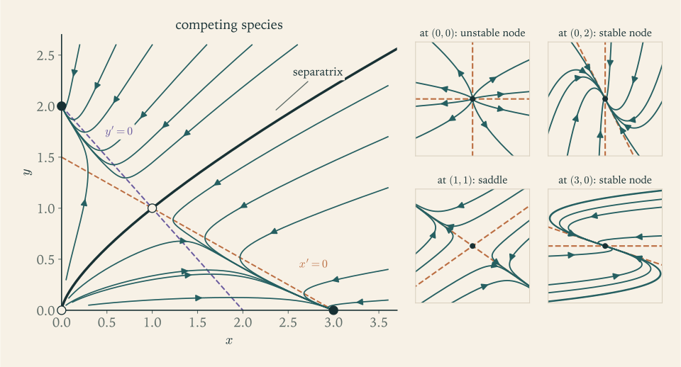
Nullclines. \(x'=0\) on the line \(x=0\) and on the line \(x+2y=3\) . \(y'=0\) on the line \(y=0\) and on the line \(x+y=2\) .
Equilibria. Intersect each \(x\) -nullcline with each \(y\) -nullcline. From \(x=0\) and \(y=0\) : \((0,0)\) . From \(x=0\) and \(x+y=2\) : \((0,2)\) . From \(x+2y=3\) and \(y=0\) : \((3,0)\) . From \(x+2y=3\) and \(x+y=2\) : subtracting gives \(y=1\) , then \(x=1\) , so \((1,1)\) .
Directions. In the quadrant \(x>0\) , \(y>0\) the sign of \(x'\) is the sign of \(3-x-2y\) , positive below the line \(x+2y=3\) ; the sign of \(y'\) is that of \(2-x-y\) , positive below the line \(x+y=2\) . The two lines cross at \((1,1)\) and cut the quadrant into four regions. Near the origin both populations grow. Far out both shrink. In the two wedge-shaped regions between the lines, one species grows while the other declines: in the wedge next to the \(x\) -axis, \(x'>0\) and \(y'<0\) , and in the wedge next to the \(y\) -axis, \(x'<0\) and \(y'>0\) .
The axes are made of trajectories: if \(y=0\) initially then \(y\) stays \(0\) , and \(x\) obeys the logistic equation \(x'=x(3-x)\) . Because trajectories cannot cross, a solution that starts with both populations positive keeps both positive for all time. The sign information suggests that trajectories in the lower wedge head for \((3,0)\) and those in the upper wedge for \((0,2)\) . What happens near \((1,1)\) needs a closer look.
8.2 What stability means
On the phase line of Chapter 1, “stable” meant that nearby solutions approach the equilibrium. In the plane a third possibility appears, already visible at a centre: nearby solutions may stay nearby without approaching. The definitions separate the two ideas.
Definition 8.2 (stability). Let \(\mathbf x^{*}\) be an equilibrium of \(\mathbf x'=\mathbf F(\mathbf x)\) .
It is stable if for every \(\varepsilon>0\) there is a \(\delta>0\) such that every solution with \(\lVert\mathbf x(0)-\mathbf x^{*}\rVert<\delta\) exists for all \(t\ge0\) and satisfies \(\lVert\mathbf x(t)-\mathbf x^{*}\rVert<\varepsilon\) for all \(t\ge0\) .
It is asymptotically stable if it is stable and there is a \(\delta_0>0\) such that every solution with \(\lVert\mathbf x(0)-\mathbf x^{*}\rVert<\delta_0\) satisfies \(\mathbf x(t)\to\mathbf x^{*}\) as \(t\to\infty\) .
It is unstable if it is not stable.
Stability is a promise about staying close: to remain within \(\varepsilon\) , start within \(\delta\) . Asymptotic stability adds convergence. For the linear systems of Chapter 7 the origin is asymptotically stable when both eigenvalues have negative real part (Theorem 7.8), stable but not asymptotically stable at a centre, and unstable at saddles and at unstable nodes and spirals. The set of all initial points whose solutions converge to an asymptotically stable equilibrium is its basin of attraction.
8.3 Linearization
Near an equilibrium \(\mathbf x^{*}=(x^{*},y^{*})\) write \(\mathbf x=\mathbf x^{*}+\mathbf u\) . Since \(\mathbf F(\mathbf x^{*})=\mathbf 0\) and \(\mathbf F\) is differentiable,
where the remainder is small compared with \(\mathbf u\) : \(\lVert\mathbf R(\mathbf u)\rVert/\lVert\mathbf u\rVert\to0\) as \(\mathbf u\to\mathbf 0\) . The matrix \(J\) of partial derivatives at the equilibrium is the Jacobian matrix, and \(\mathbf u'=J\mathbf u\) is the linearization of the system at \(\mathbf x^{*}\) . For small \(\mathbf u\) the deviation obeys \(\mathbf u'=J\mathbf u+\mathbf R(\mathbf u)\) , a linear system with a small perturbation. Whether the perturbation matters depends on the eigenvalues of \(J\) .
Theorem 8.3 (stability by linearization). Let \(\mathbf F\) have continuous first partial derivatives near an equilibrium \(\mathbf x^{*}\) of the planar system \(\mathbf x'=\mathbf F(\mathbf x)\) , with Jacobian matrix \(J\) there.
(a) If every eigenvalue of \(J\) has negative real part, \(\mathbf x^{*}\) is asymptotically stable.
(b) If some eigenvalue of \(J\) has positive real part, \(\mathbf x^{*}\) is unstable.
(c) If no eigenvalue has positive real part but some eigenvalue has real part zero, the linearization does not determine the stability of \(\mathbf x^{*}\) .
Proof of (a). By Theorem 7.8 there are \(C\ge1\) and \(\alpha>0\) with \(\lVert e^{tJ}\mathbf v\rVert\le Ce^{-\alpha t}\lVert\mathbf v\rVert\) for \(t\ge0\) . Put \(\eta=\alpha/(2C)\) and choose \(\rho>0\) so small that \(\lVert\mathbf R(\mathbf u)\rVert\le\eta\lVert\mathbf u\rVert\) whenever \(\lVert\mathbf u\rVert\le\rho\) .
Let \(\mathbf u\) be a solution of \(\mathbf u'=J\mathbf u+\mathbf R(\mathbf u)\) with \(\lVert\mathbf u(0)\rVert<\rho/C\) . Treating \(\mathbf R(\mathbf u(s))\) as a forcing term, variation of constants (Theorem 7.9) gives
As long as \(\lVert\mathbf u(s)\rVert\le\rho\) on \([0,t]\) ,
Multiply by \(e^{\alpha t}\) and set \(w(t)=e^{\alpha t}\lVert\mathbf u(t)\rVert\) : then \(w(t)\le C\lVert\mathbf u(0)\rVert+C\eta\int_0^tw(s)\,ds\) . Grönwall’s inequality (Lemma 3.6) gives \(w(t)\le C\lVert\mathbf u(0)\rVert e^{C\eta t}\) , that is,
The right side is less than \(\rho\) . So the solution cannot reach the circle \(\lVert\mathbf u\rVert=\rho\) : at the first time it did, the estimate, valid up to that time, would give a norm strictly less than \(\rho\) . Hence the solution stays in the disc of radius \(\rho\) , exists for all \(t\ge0\) by Theorem 3.11, and obeys the estimate for all \(t\ge0\) . The estimate shows stability, with \(\delta=\min(\rho,\varepsilon)/C\) , and convergence to \(\mathbf 0\) at an exponential rate.
The proof shows more than the statement: near an equilibrium whose linearization is asymptotically stable, solutions converge exponentially, at any rate slower than the linear one. Part (b) is true for the same reason turned around, that the linear growth along an unstable direction outruns the remainder, but its proof is longer and is omitted. Part (c) is demonstrated by Example 8.3 below.
An equilibrium at which no eigenvalue of \(J\) has zero real part is called hyperbolic. For hyperbolic equilibria much more than stability is preserved. Two results are quoted here without proof. The Hartman–Grobman theorem states that near a hyperbolic equilibrium the phase portrait of the nonlinear system is a continuous distortion of the phase portrait of its linearization: a saddle of the linearization is a saddle of the nonlinear system, a sink is a sink, and a source is a source. The stable manifold theorem adds that at a saddle exactly two trajectories arrive and two leave, and that they are tangent at the equilibrium to the eigenvector lines of \(J\) . If \(\mathbf F\) is twice continuously differentiable, nodes also remain nodes and spirals remain spirals.
Example 8.2: The four equilibria of the competition model
For Example 8.1, \(f=3x-x^2-2xy\) and \(g=2y-xy-y^2\) , so
At \((0,0)\) : \(J=\begin{pmatrix}3&0\\0&2\end{pmatrix}\) , eigenvalues \(3\) and \(2\) . An unstable node: two small populations both grow.
At \((3,0)\) : \(J=\begin{pmatrix}-3&-6\\0&-1\end{pmatrix}\) , eigenvalues \(-3\) and \(-1\) . A stable node: species \(x\) alone at its carrying capacity, and a small invasion by \(y\) dies out.
At \((0,2)\) : \(J=\begin{pmatrix}-1&0\\-2&-2\end{pmatrix}\) , eigenvalues \(-1\) and \(-2\) . A stable node: species \(y\) alone.
At \((1,1)\) : \(J=\begin{pmatrix}-1&-2\\-1&-1\end{pmatrix}\) , with \(\tau=-2\) and \(\Delta=-1<0\) . A saddle, with eigenvalues \(-1\pm\sqrt2\) , about \(0.414\) and \(-2.414\) . The stable direction, belonging to \(-1-\sqrt2\) , is \((\sqrt2,1)\) , and the unstable direction is \((\sqrt2,-1)\) .
All four equilibria are hyperbolic, so Theorem 8.3 and the remarks after it apply to each. Coexistence at \((1,1)\) is unstable. The two trajectories that arrive at the saddle form a curve, the separatrix, running from the origin through \((1,1)\) and on to infinity. It divides the positive quadrant into the basins of attraction of the two stable nodes. Populations starting below the separatrix end at \((3,0)\) , and those above it at \((0,2)\) : whichever species has the initial advantage, in the sense defined by that curve, eliminates the other.
8.4 What linearization cannot decide
When \(J\) has an eigenvalue with zero real part, the linear terms neither attract nor repel along some direction, and the neglected remainder decides the outcome.
Example 8.3: Three systems with one linearization
For a constant \(a\) consider
The origin is an equilibrium, and the Jacobian there is \(\begin{pmatrix}0&-1\\1&0\end{pmatrix}\) for every \(a\) , since the added terms are cubic. Its eigenvalues are \(\pm i\) : the linearization is a centre, with every trajectory a circle.
For the nonlinear system let \(r^2=x^2+y^2\) . Then
If \(a=0\) the system is linear and \(r\) is constant: a centre. If \(a<0\) then \(r\) decreases, and solving \(r'=ar^3\) gives \(r(t)=r_0/\sqrt{1+2\lvert a\rvert r_0^2t}\to0\) : the origin is asymptotically stable, and trajectories spiral in. If \(a>0\) then \(r(t)=r_0/\sqrt{1-2ar_0^2t}\) , which increases and becomes infinite at \(t=1/(2ar_0^2)\) : the origin is unstable.
The same linearization accompanies a stable centre, an asymptotically stable spiral, and an unstable one. The decay for \(a<0\) is like \(t^{-1/2}\) , slower than any exponential, which is the signature of a non-hyperbolic equilibrium.
Common mistake. Reading the stability of a nonlinear equilibrium from a linearization with purely imaginary or zero eigenvalues. “The Jacobian has eigenvalues \(\pm i\) , so the equilibrium is a centre and solutions are periodic” is an invalid inference, as the example shows. In case (c) of Theorem 8.3 the only correct statement from linearization alone is “no conclusion”. Something else must be used: a conserved quantity, a Lyapunov function, or polar coordinates.
8.5 Conserved quantities and the pendulum
Definition 8.4 (conserved quantity). A continuously differentiable function \(E(x,y)\) , not constant on any open set, is a conserved quantity of the system \(x'=f\) , \(y'=g\) if it is constant along every solution, that is, if
at every point.
Each trajectory then lies in a single level set of \(E\) , so the phase portrait is, up to the direction of travel, the contour map of \(E\) . A system with a conserved quantity cannot have an asymptotically stable equilibrium (Exercise 12), but it can have stable ones.
Proposition 8.5 (a strict minimum of a conserved quantity is stable). If \(E\) is a conserved quantity and has a strict local minimum at an equilibrium \(\mathbf x^{*}\) , then \(\mathbf x^{*}\) is stable.
This is a special case of Theorem 8.6 below, with \(V=E-E(\mathbf x^{*})\) , and is proved there.
Example 8.4: The pendulum, without and with friction
With \(x=\theta\) and \(y=\theta'\) the pendulum equation \(\theta''+\sin\theta=0\) is
Equilibria and linearization. The equilibria are \((k\pi,0)\) . The Jacobian is \(\begin{pmatrix}0&1\\-\cos x&0\end{pmatrix}\) . At \((\pi,0)\) , the upright position, it is \(\begin{pmatrix}0&1\\1&0\end{pmatrix}\) with eigenvalues \(\pm1\) and eigenvectors \((1,1)\) and \((1,-1)\) : a saddle, hence unstable. At \((0,0)\) , hanging straight down, it is \(\begin{pmatrix}0&1\\-1&0\end{pmatrix}\) with eigenvalues \(\pm i\) : no conclusion.
Energy. Let \(E(x,y)=\tfrac12y^2+1-\cos x\) , kinetic plus potential energy. Then \(E_x\,x'+E_y\,y'=\sin x\cdot y+y\cdot(-\sin x)=0\) , so \(E\) is conserved. At \((0,0)\) , \(E=0\) , and \(E>0\) at all nearby points, since \(1-\cos x>0\) for \(0<\lvert x\rvert<2\pi\) . By Proposition 8.5 the downward equilibrium is stable. It is a true centre: for \(0<E<2\) the level set near the origin is a closed curve containing no equilibrium, so the solution on it is periodic.
The global picture. The level \(E=2\) passes through the saddles \((\pm\pi,0)\) . On it \(\tfrac12y^2=1+\cos x=2\cos^2(x/2)\) , so it consists of the curves \(y=\pm2\cos(x/2)\) , the separatrices. Inside them, \(0<E<2\) , the pendulum swings back and forth. Outside them, \(E>2\) , the velocity never vanishes and the pendulum rotates, clockwise or counterclockwise for ever. On a separatrix it approaches the upright position as \(t\to\infty\) without reaching it.
Period. The linear approximation gives period \(2\pi\approx6.283\) for every amplitude. The true period of the oscillation with amplitude \(\theta_0\) is \(4\int_0^{\theta_0}d\theta/\sqrt{2(\cos\theta-\cos\theta_0)}\) , from \(\tfrac12(\theta')^2=\cos\theta-\cos\theta_0\) . For \(\theta_0=\pi/2\) numerical integration gives \(7.416\) , eighteen percent longer, and the period tends to infinity as \(\theta_0\to\pi\) .
Friction. With damping, \(\theta''+c\,\theta'+\sin\theta=0\) with \(c>0\) , the system is \(x'=y\) , \(y'=-\sin x-cy\) , and now \(E'=y\,(-cy)=-cy^2\le0\) : energy is lost whenever the pendulum moves. The Jacobian at \((0,0)\) is \(\begin{pmatrix}0&1\\-1&-c\end{pmatrix}\) , with \(\tau=-c<0\) and \(\Delta=1>0\) : asymptotically stable by Theorem 8.3, a spiral if \(c<2\) . The upright equilibrium remains a saddle, since \(\Delta=-1\) .
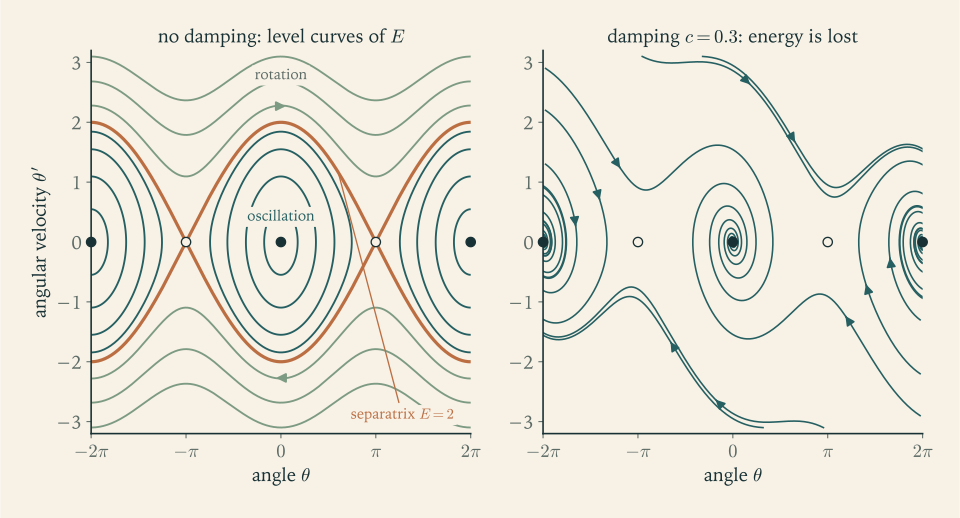
The two panels of Figure 8.2 show how fragile a centre is. An arbitrarily small friction term converts every closed orbit into a spiral and each centre into a sink, while the saddles, being hyperbolic, are unaffected. This is Theorem 8.3(c) from another angle: a non-hyperbolic equilibrium is one whose character can be changed by an arbitrarily small change in the equations.
8.6 Lyapunov functions
The energy argument does not need the function to be an energy, or to be conserved. It needs a function with a strict minimum at the equilibrium that does not increase along solutions. For a continuously differentiable \(V(x,y)\) and a system \(x'=f\) , \(y'=g\) , write
By the chain rule this is the rate of change of \(V\) along the solution through the point, and it is computed from \(V\) and the equations alone, without knowing any solution.
Theorem 8.6 (Lyapunov’s direct method). Let \(\mathbf x^{*}\) be an equilibrium of \(\mathbf x'=\mathbf F(\mathbf x)\) and let \(V\) be continuously differentiable on an open set \(U\) containing \(\mathbf x^{*}\) , with \(V(\mathbf x^{*})=0\) and \(V(\mathbf x)>0\) for all other \(\mathbf x\in U\) .
(a) If \(\dot V\le0\) on \(U\) , then \(\mathbf x^{*}\) is stable.
(b) If \(\dot V<0\) on \(U\) except at \(\mathbf x^{*}\) , then \(\mathbf x^{*}\) is asymptotically stable.
Proof. (a) Let \(\varepsilon>0\) be small enough that the closed disc \(B_\varepsilon\) of radius \(\varepsilon\) about \(\mathbf x^{*}\) lies in \(U\) . On its boundary circle, a closed bounded set not containing \(\mathbf x^{*}\) , the continuous positive function \(V\) has a minimum \(m>0\) . Since \(V\) is continuous and \(V(\mathbf x^{*})=0\) , there is \(\delta<\varepsilon\) with \(V<m\) on the disc of radius \(\delta\) . Let a solution start in that disc. Along it \(\frac{d}{dt}V(\mathbf x(t))=\dot V\le0\) , so \(V(\mathbf x(t))\le V(\mathbf x(0))<m\) as long as the solution stays in \(U\) . It therefore cannot reach the circle of radius \(\varepsilon\) , where \(V\ge m\) . Being confined to \(B_\varepsilon\) , it exists for all \(t\ge0\) (Theorem 3.11) and stays within \(\varepsilon\) of \(\mathbf x^{*}\) .
(b) By (a) the equilibrium is stable; take a solution as above, confined to \(B_\varepsilon\) . The function \(V(\mathbf x(t))\) is nonincreasing and nonnegative, so it has a limit \(c\ge0\) . Suppose \(c>0\) . The set \(K\) of points of \(B_\varepsilon\) with \(V\ge c\) is closed and bounded and does not contain \(\mathbf x^{*}\) , so on it the continuous function \(\dot V\) has a maximum \(-\mu<0\) . The solution stays in \(K\) , hence \(V(\mathbf x(t))\le V(\mathbf x(0))-\mu t\) , which becomes negative, a contradiction. So \(V(\mathbf x(t))\to0\) . Finally, if \(\mathbf x(t)\) did not tend to \(\mathbf x^{*}\) , there would be \(\sigma>0\) and times \(t_k\to\infty\) with \(\lVert\mathbf x(t_k)-\mathbf x^{*}\rVert\ge\sigma\) ; on the closed bounded set \(\sigma\le\lVert\mathbf x-\mathbf x^{*}\rVert\le\varepsilon\) the function \(V\) has a positive minimum, contradicting \(V(\mathbf x(t_k))\to0\) .
A function \(V\) as in the theorem is a Lyapunov function. Geometrically, the level curves of \(V\) near \(\mathbf x^{*}\) are closed curves around it, and \(\dot V<0\) says every trajectory crosses them inward. Unlike linearization, the method gives explicit regions: any sublevel set \(\{V\le k\}\) that is a closed bounded subset of \(U\) lies in the basin of attraction in case (b). There is no general recipe for finding \(V\) . Physical energy, the squared distance \(x^2+y^2\) , and quadratic forms \(ax^2+by^2\) with constants chosen to cancel unwanted terms are the usual first attempts.
Example 8.5: Stability where linearization is silent
Consider \(x'=-y-x^3\) , \(y'=x-y^3\) . The Jacobian at the origin is \(\begin{pmatrix}0&-1\\1&0\end{pmatrix}\) , eigenvalues \(\pm i\) : no conclusion from Theorem 8.3.
Try \(V=x^2+y^2\) . Then
which is negative everywhere except at the origin. By Theorem 8.6(b), with \(U\) the whole plane, the origin is asymptotically stable, and since every sublevel set of \(V\) is a disc, every solution converges to it.
The rate can be estimated. Since \(x^4+y^4\ge\tfrac12(x^2+y^2)^2\) , we have \(\dot V\le-V^2\) along solutions, and comparing with \(v'=-v^2\) gives \(V(t)\le V(0)/(1+V(0)\,t)\) . The squared distance to the origin decays at least like \(1/t\) : convergence is certain but slow.
8.7 Closed orbits
Linear systems have periodic solutions only at a centre, where they come in a continuous family. Nonlinear systems can have an isolated periodic solution that attracts its neighbours, something with no linear counterpart.
Example 8.6: A limit cycle
Consider
With \(r^2=x^2+y^2\) , the computation of Example 8.3 gives \(r\,r'=x\,x'+y\,y'=r^2-r^4\) , so \(r'=r(1-r^2)\) . For the polar angle, \(\theta'=(x\,y'-y\,x')/r^2=(x^2+y^2)/r^2=1\) . In polar coordinates the system decouples:
The first equation is autonomous in one variable, and its phase line on \(r\ge0\) has an unstable equilibrium at \(r=0\) and a stable one at \(r=1\) . So the origin is an unstable equilibrium of the planar system, in agreement with its Jacobian \(\begin{pmatrix}1&-1\\1&1\end{pmatrix}\) , whose eigenvalues are \(1\pm i\) . The circle \(r=1\) is a closed trajectory, traversed counterclockwise with period \(2\pi\) , and every other trajectory except the origin spirals toward it, from inside or from outside. Explicitly, \(r(t)^2=1/\bigl(1+(r_0^{-2}-1)e^{-2t}\bigr)\) .
A closed trajectory that nearby trajectories approach is a stable limit cycle. It represents a self-sustained oscillation whose amplitude and period are set by the system and not by the initial conditions, as in a heartbeat or an electronic oscillator. A linear centre is different in kind: there the amplitude is whatever the initial condition makes it, and the smallest friction destroys the oscillation.
In the plane this is essentially the full list of long-term behaviours. A theorem of Poincaré and Bendixson, stated here without proof, says that a trajectory of a planar autonomous system that stays in a closed bounded region containing no equilibria must approach a closed orbit. Trajectories in the plane are constrained by the fact that they cannot cross. In three or more dimensions that constraint loses its force, and bounded trajectories can wander for ever without settling into any pattern.
The course began with the question of what a differential equation asserts and ends with the observation that the most informative answer is often a picture and a handful of eigenvalues. Formulas, where they exist, give numbers. The qualitative theory says which questions can be answered with certainty when no formula exists.
Exercises
-
For the predator-prey system \(x'=x\,(1-y)\) , \(y'=y\,(x-1)\) find the equilibria and their linearizations, show that \(H=x-\ln x+y-\ln y\) is conserved in the quadrant \(x,y>0\) , and use it to settle the stability of the equilibrium that linearization cannot decide.
Solution
Equilibria. \(x(1-y)=0\) and \(y(x-1)=0\) . If \(x=0\) the second equation gives \(y=0\) ; if \(y=1\) it gives \(x=1\) . So the equilibria are \((0,0)\) and \((1,1)\) .
Linearization. \(J=\begin{pmatrix}1-y&-x\\y&x-1\end{pmatrix}\) . At \((0,0)\) it is \(\begin{pmatrix}1&0\\0&-1\end{pmatrix}\) , a saddle, so the origin is unstable by Theorem 8.3(b). At \((1,1)\) it is \(\begin{pmatrix}0&-1\\1&0\end{pmatrix}\) with eigenvalues \(\pm i\) , so Theorem 8.3 gives no conclusion.
Conserved quantity. With \(H_x=1-1/x\) and \(H_y=1-1/y\) ,
\[ H_x\,x'+H_y\,y'=\Bigl(1-\frac1x\Bigr)x\,(1-y)+\Bigl(1-\frac1y\Bigr)y\,(x-1)=(x-1)(1-y)+(y-1)(x-1)=0 . \]Stability of \((1,1)\) . The function \(h(s)=s-\ln s\) on \(s>0\) has \(h'(s)=1-1/s\) and \(h''(s)=1/s^2>0\) , so it has a strict global minimum at \(s=1\) . Therefore \(H=h(x)+h(y)\) has a strict minimum at \((1,1)\) , and by Proposition 8.5 that equilibrium is stable. The level sets of \(H\) near \((1,1)\) are closed curves, so the populations cycle periodically around the equilibrium. By Exercise 8.12 the equilibrium is not asymptotically stable. The linearization’s centre happens to be correct here, but only the conserved quantity proves it.
-
Write \(x''+\tfrac12x'=x-x^3\) as a system, find its three equilibria, and classify each by its Jacobian matrix, stating which theorem justifies each conclusion.
Answer
\(x'=y\) , \(y'=x-x^3-\tfrac12y\) ; equilibria \((0,0)\) and \((\pm1,0)\) ; \(J=\begin{pmatrix}0&1\\1-3x^2&-\tfrac12\end{pmatrix}\) . At \((0,0)\) : \(\Delta=-1\) , a saddle with eigenvalues about \(0.781\) and \(-1.281\) , unstable by Theorem 8.3(b). At \((\pm1,0)\) : \(\tau=-\tfrac12\) , \(\Delta=2\) , \(\tau^2-4\Delta<0\) , stable spirals, asymptotically stable by Theorem 8.3(a).
-
For the competition model \(x'=x\,(3-2x-y)\) , \(y'=y\,(3-x-2y)\) find the four equilibria, classify each, and explain how the outcome differs from that of Example 8.2.
Solution
The \(x\) -nullclines are \(x=0\) and \(2x+y=3\) ; the \(y\) -nullclines are \(y=0\) and \(x+2y=3\) . Intersections: \((0,0)\) ; \((0,\tfrac32)\) from \(x=0\) , \(x+2y=3\) ; \((\tfrac32,0)\) from \(y=0\) , \(2x+y=3\) ; and \((1,1)\) from the two slanted lines.
With \(f=3x-2x^2-xy\) and \(g=3y-xy-2y^2\) ,
\[ J=\begin{pmatrix}3-4x-y&-x\\-y&3-x-4y\end{pmatrix}. \]At \((0,0)\) : \(J=3I\) , an unstable node. At \((\tfrac32,0)\) : \(J=\begin{pmatrix}-3&-\tfrac32\\0&\tfrac32\end{pmatrix}\) , eigenvalues \(-3\) and \(\tfrac32\) , a saddle. At \((0,\tfrac32)\) : \(J=\begin{pmatrix}\tfrac32&0\\-\tfrac32&-3\end{pmatrix}\) , eigenvalues \(\tfrac32\) and \(-3\) , a saddle. At \((1,1)\) : \(J=\begin{pmatrix}-2&-1\\-1&-2\end{pmatrix}\) , with \(\tau=-4\) , \(\Delta=3\) , eigenvalues \(-1\) and \(-3\) , a stable node.
All four are hyperbolic, so Theorem 8.3 applies. Here the coexistence equilibrium \((1,1)\) is asymptotically stable and the single-species equilibria are unstable: each species alone can be invaded by the other. In Example 8.2 it was the reverse. The difference is the strength of competition between the species relative to competition within each: in this exercise each species limits itself (coefficient \(2\) ) more than it limits its rival (coefficient \(1\) ), and they coexist; in Example 8.2 species \(y\) depresses \(x\) more strongly than \(x\) depresses itself, and one species is excluded.
-
Using Definition 8.2 directly, decide whether the origin is stable, asymptotically stable, or unstable for (a) \(x'=-x\) , \(y'=-2y\) ; (b) \(x'=y\) , \(y'=-x\) ; (c) \(x'=x\) , \(y'=-y\) ; (d) \(x'=0\) , \(y'=-y\) , and explain why case (d) is not covered by Theorem 7.7.
Answer
(a) Asymptotically stable: \(\lVert\mathbf x(t)\rVert\le e^{-t}\lVert\mathbf x(0)\rVert\) . (b) Stable, not asymptotically: solutions move on circles, so \(\delta=\varepsilon\) works and nothing converges. (c) Unstable: solutions with \(x(0)\ne0\) leave every disc. (d) Stable, not asymptotically: the solution is \((x_0,y_0e^{-t})\) , which stays within its initial distance of the origin and tends to \((x_0,0)\) , not to the origin. Here \(\det A=0\) and every point of the \(x\) -axis is an equilibrium; Theorem 7.7 assumes \(\Delta\ne0\) .
-
For \(x'=-y+x\,(x^2+y^2-1)\) , \(y'=x+y\,(x^2+y^2-1)\) derive the equations for \(r\) and \(\theta\) , classify the origin by linearization, identify the closed orbit and say whether it is a stable limit cycle, and describe the basin of attraction of the origin.
Solution
Polar form. With \(r^2=x^2+y^2\) : \(r\,r'=x\,x'+y\,y'=-xy+x^2(r^2-1)+xy+y^2(r^2-1)=r^2(r^2-1)\) , so \(r'=r\,(r^2-1)\) . And \(\theta'=(x\,y'-y\,x')/r^2=(x^2+y^2)/r^2=1\) .
The origin. The Jacobian at the origin is \(\begin{pmatrix}-1&-1\\1&-1\end{pmatrix}\) , with \(\tau=-2\) , \(\Delta=2\) , eigenvalues \(-1\pm i\) : a stable spiral, asymptotically stable by Theorem 8.3(a).
The closed orbit. The equation \(r'=r(r^2-1)\) has equilibria \(r=0\) and \(r=1\) on \(r\ge0\) . The circle \(r=1\) is a closed trajectory. But \(r'<0\) for \(0<r<1\) and \(r'>0\) for \(r>1\) , so trajectories on both sides move away from the circle. It is an unstable closed orbit, not a stable limit cycle; compare Example 8.6, where the signs are opposite.
Basin. A trajectory starting with \(0<r_0<1\) has \(r\) decreasing, and \(r\to0\) by Proposition 1.6 applied to the \(r\) -equation. A trajectory starting on the circle stays on it, and one starting outside has \(r\) increasing without bound, in fact to infinity in finite time, since \(r'\ge r^3-r\) grows cubically. So the basin of attraction of the origin is exactly the open unit disc. The unstable closed orbit is the boundary of the basin, the planar analogue of the threshold equilibrium in Example 1.5.
-
Show that \(V=x^2+y^2\) is a Lyapunov function for \(x'=-x+y^2\) , \(y'=-y-xy\) at the origin, find \(V\) along solutions explicitly, and state the basin of attraction.
Answer
\(\dot V=2x(-x+y^2)+2y(-y-xy)=-2(x^2+y^2)=-2V\) , so \(V(t)=V(0)e^{-2t}\) . \(V\) is positive except at the origin and \(\dot V<0\) except there; every solution converges, so the basin is the whole plane.
-
For \(x'=y-x^3\) , \(y'=-2x-y^3\) show that linearization at the origin is inconclusive, then find constants \(a,b>0\) for which \(V=ax^2+by^2\) is a Lyapunov function proving asymptotic stability.
Solution
The Jacobian at the origin is \(\begin{pmatrix}0&1\\-2&0\end{pmatrix}\) , since the cubic terms have zero derivative there. Its trace is \(0\) and determinant \(2\) , so the eigenvalues are \(\pm i\sqrt2\) , purely imaginary. This is case (c) of Theorem 8.3: no conclusion.
Try \(V=ax^2+by^2\) with \(a,b>0\) , which is zero at the origin and positive elsewhere. Then
\[ \dot V=2ax\,(y-x^3)+2by\,(-2x-y^3)=(2a-4b)\,xy-2a\,x^4-2b\,y^4 . \]The term in \(xy\) has no definite sign, so choose the constants to remove it: \(a=2b\) . With \(b=1\) , \(a=2\) :
\[ V=2x^2+y^2,\qquad\dot V=-4x^4-2y^4 , \]which is negative except at the origin. By Theorem 8.6(b) the origin is asymptotically stable, and because the sublevel sets of \(V\) are bounded ellipses filling the plane, every solution converges to it. The weights in \(V\) are those of the conserved quantity \(2x^2+y^2\) of the linear part \(x'=y\) , \(y'=-2x\) ; the cubic terms then supply the dissipation.
-
A student linearizes \(x'=y+x^3\) , \(y'=-x+y^3\) at the origin, finds eigenvalues \(\pm i\) , and concludes that the origin is a stable centre. Explain the error in the inference and determine the true stability using \(V=x^2+y^2\) .
Solution
The error. The Jacobian at the origin is \(\begin{pmatrix}0&1\\-1&0\end{pmatrix}\) , eigenvalues \(\pm i\) . These have zero real part, so the equilibrium is not hyperbolic and Theorem 8.3(c) applies: the linearization determines nothing about the nonlinear system. The student has transferred the conclusion “centre” from the linear system to the nonlinear one, which is legitimate only for hyperbolic equilibria.
The truth. With \(V=x^2+y^2\) ,
\[ \dot V=2x\,(y+x^3)+2y\,(-x+y^3)=2\,(x^4+y^4)>0 \]away from the origin. So the squared distance from the origin strictly increases along every nonzero solution. That alone shows the origin is not asymptotically stable. For instability, use \(x^4+y^4\ge\tfrac12(x^2+y^2)^2\) , which gives \(\dot V\ge V^2\) along solutions. Then \(\frac{d}{dt}(-1/V)\ge1\) , so \(V(t)\ge V(0)/(1-V(0)\,t)\) : however small \(V(0)>0\) is, the solution leaves any given disc before time \(1/V(0)\) . Given \(\varepsilon>0\) , no \(\delta\) can keep solutions within \(\varepsilon\) . The origin is unstable, with trajectories spiralling slowly outward.
-
For the damped pendulum \(\theta''+\tfrac12\theta'+\sin\theta=0\) classify the equilibria \((0,0)\) and \((\pi,0)\) , give the eigenvalues at the saddle, and verify that the energy \(E=\tfrac12y^2+1-\cos x\) satisfies \(E'=-\tfrac12y^2\) .
Answer
The system is \(x'=y\) , \(y'=-\sin x-\tfrac12y\) . At \((0,0)\) : \(J=\begin{pmatrix}0&1\\-1&-\tfrac12\end{pmatrix}\) , \(\tau=-\tfrac12\) , \(\Delta=1\) , a stable spiral. At \((\pi,0)\) : \(J=\begin{pmatrix}0&1\\1&-\tfrac12\end{pmatrix}\) , \(\Delta=-1\) , a saddle with eigenvalues \(\tfrac14(-1\pm\sqrt{17})\approx0.781\) and \(-1.281\) . \(E'=\sin x\cdot y+y\,(-\sin x-\tfrac12y)=-\tfrac12y^2\) .
-
Verify that \(x(t)=4\arctan(e^{t})-\pi\) , \(y(t)=x'(t)\) is a solution of the undamped pendulum system that lies on the separatrix \(E=2\) , and find its limits as \(t\to\infty\) and \(t\to-\infty\) .
Solution
First equation. Differentiating, \(x'(t)=\dfrac{4e^{t}}{1+e^{2t}}=\dfrac{2}{\cosh t}\) , and this is \(y(t)\) by definition, so \(x'=y\) holds.
Second equation. We need \(y'=-\sin x\) . On one side, \(y'=-\dfrac{2\sinh t}{\cosh^2t}\) . On the other, let \(\psi=\arctan(e^{t})\) , so \(x/2=2\psi-\pi/2\) . Then
\[ \cos\frac x2=\sin2\psi=\frac{2\tan\psi}{1+\tan^2\psi}=\frac{2e^{t}}{1+e^{2t}}=\frac{1}{\cosh t},\qquad\sin\frac x2=-\cos2\psi=\frac{e^{2t}-1}{e^{2t}+1}=\tanh t . \]Hence \(\sin x=2\sin\frac x2\cos\frac x2=\dfrac{2\tanh t}{\cosh t}=\dfrac{2\sinh t}{\cosh^2t}\) , and \(y'=-\sin x\) as required.
Energy. \(E=\tfrac12y^2+1-\cos x=\dfrac{2}{\cosh^2t}+2\sin^2\dfrac x2=\dfrac{2}{\cosh^2t}+2\tanh^2t=2\) . The solution lies on the upper separatrix \(y=2\cos(x/2)\) .
Limits. As \(t\to\infty\) , \(\arctan(e^{t})\to\pi/2\) , so \(x\to\pi\) and \(y=2/\cosh t\to0\) . As \(t\to-\infty\) , \(\arctan(e^{t})\to0\) , so \(x\to-\pi\) and \(y\to0\) . The trajectory joins the saddle \((-\pi,0)\) to the saddle \((\pi,0)\) and takes infinitely long at both ends: the pendulum leaves the upright position infinitely slowly, swings through the bottom at \(t=0\) with speed \(2\) , and climbs back to upright without ever arriving.
-
Using conservation of energy, show that a pendulum released from rest at angle \(\theta_0\in(0,\pi)\) has period \(T=4\displaystyle\int_0^{\theta_0}\frac{d\theta}{\sqrt{2(\cos\theta-\cos\theta_0)}}\) , and evaluate \(T\) numerically for \(\theta_0=\pi/2\) by any method, comparing with \(2\pi\) .
Answer
From \(\tfrac12(\theta')^2+1-\cos\theta=1-\cos\theta_0\) , \(\theta'=\pm\sqrt{2(\cos\theta-\cos\theta_0)}\) ; a quarter period is the time to go from \(\theta=0\) to \(\theta_0\) , which gives the formula. For \(\theta_0=\pi/2\) , \(T\approx7.416\) , against \(2\pi\approx6.283\) .
-
Prove that a planar system with a conserved quantity in the sense of Definition 8.4 has no asymptotically stable equilibrium.
Solution
Suppose \(E\) is a conserved quantity and \(\mathbf x^{*}\) is an asymptotically stable equilibrium. Then there is \(\delta_0>0\) such that every solution starting in the disc \(D\) of radius \(\delta_0\) about \(\mathbf x^{*}\) converges to \(\mathbf x^{*}\) .
Take any point \(\mathbf p\in D\) and the solution \(\mathbf x(t)\) with \(\mathbf x(0)=\mathbf p\) . Because \(E\) is conserved, \(E(\mathbf x(t))=E(\mathbf p)\) for all \(t\ge0\) . Because \(E\) is continuous and \(\mathbf x(t)\to\mathbf x^{*}\) , also \(E(\mathbf x(t))\to E(\mathbf x^{*})\) . A constant function of \(t\) that has a limit equals that limit, so \(E(\mathbf p)=E(\mathbf x^{*})\) .
This holds for every \(\mathbf p\in D\) , so \(E\) is constant on the open disc \(D\) . That contradicts the requirement in Definition 8.4 that a conserved quantity is not constant on any open set. Hence no equilibrium is asymptotically stable. The requirement is what gives the definition content: without it every system would have the constant functions as conserved quantities. The same argument shows that such a system has no stable limit cycles and no sources: trajectories cannot all funnel into, or out of, a lower-dimensional set while each keeps its own value of \(E\) .
-
A gradient system has the form \(\mathbf x'=-\nabla V(\mathbf x)\) for a twice continuously differentiable function \(V\) . Prove that \(V\) is strictly decreasing along every nonconstant solution and deduce that a gradient system has no periodic solutions other than equilibria.
Hint
Compute \(\frac{d}{dt}V(\mathbf x(t))=\nabla V\cdot\mathbf x'=-\lVert\nabla V\rVert^2\) . On a periodic solution \(V\) would return to its starting value after one period.
-
For \(x'=y-x^2\) , \(y'=x-y\) draw the nullclines, mark the signs of \(x'\) and \(y'\) in each region, find the two equilibria, and classify them.
Answer
\(x'=0\) on the parabola \(y=x^2\) , with \(x'>0\) above it; \(y'=0\) on the line \(y=x\) , with \(y'>0\) below it. Equilibria \((0,0)\) and \((1,1)\) . \(J=\begin{pmatrix}-2x&1\\1&-1\end{pmatrix}\) : at \((0,0)\) , \(\Delta=-1\) , a saddle; at \((1,1)\) , \(\tau=-3\) , \(\Delta=1\) , \(\tau^2-4\Delta=5>0\) , a stable node.
-
Write the van der Pol equation \(x''+\mu\,(x^2-1)\,x'+x=0\) as a system and use the trace and determinant of the Jacobian at the origin to classify the origin for every \(\mu>0\) ; relate the result to the classification of Theorem 7.7.
Hint
The system is \(x'=y\) , \(y'=-x-\mu(x^2-1)y\) , and the Jacobian at the origin is \(\begin{pmatrix}0&1\\-1&\mu\end{pmatrix}\) , with \(\tau=\mu\) and \(\Delta=1\) . Compare \(\tau^2\) with \(4\Delta\) .
-
In the model \(x'=x\,(1-x)-xy\) , \(y'=y\,(x-\tfrac12)\) the prey \(x\) grows logistically and the predator \(y\) dies out without prey. Find the equilibria with \(x,y\ge0\) , classify each, and describe in words the long-term behaviour of populations that start with both species present.
Solution
Equilibria. From \(y\,(x-\tfrac12)=0\) : either \(y=0\) , and then \(x(1-x)=0\) gives \((0,0)\) and \((1,0)\) ; or \(x=\tfrac12\) , and then \(x(1-x-y)=0\) gives \(y=\tfrac12\) . So the equilibria are \((0,0)\) , \((1,0)\) , \((\tfrac12,\tfrac12)\) .
Jacobian. With \(f=x-x^2-xy\) and \(g=xy-\tfrac12y\) ,
\[ J=\begin{pmatrix}1-2x-y&-x\\y&x-\tfrac12\end{pmatrix}. \]At \((0,0)\) : diagonal with entries \(1\) and \(-\tfrac12\) , a saddle. At \((1,0)\) : \(\begin{pmatrix}-1&-1\\0&\tfrac12\end{pmatrix}\) , eigenvalues \(-1\) and \(\tfrac12\) , a saddle. At \((\tfrac12,\tfrac12)\) : \(\begin{pmatrix}-\tfrac12&-\tfrac12\\\tfrac12&0\end{pmatrix}\) , with \(\tau=-\tfrac12\) , \(\Delta=\tfrac14\) , and \(\tau^2-4\Delta=-\tfrac34<0\) : a stable spiral, with eigenvalues \(-\tfrac14\pm\tfrac{\sqrt3}{4}i\) .
Interpretation. All three equilibria are hyperbolic. With no predators the prey settle at the carrying capacity \(1\) , but that state is unstable to the arrival of predators, since the eigenvalue \(\tfrac12\) belongs to a direction with a predator component. Near the coexistence equilibrium both populations perform damped oscillations, the predator peak following the prey peak, with amplitude decaying like \(e^{-t/4}\) and period \(2\pi/(\sqrt3/4)\approx14.5\) . In contrast with Exercise 8.1, the logistic limitation of the prey acts like friction and turns the family of closed orbits into a sink.
-
For the system \(x'=-x+x^3\) , \(y'=-y\) find all equilibria, classify them, and determine exactly the basin of attraction of the origin.
Hint
The equations are uncoupled. Draw the phase line of \(x'=-x+x^3\) and use \(y=y_0e^{-t}\) . The Jacobian is diagonal at each equilibrium.
-
A system has the polar form \(r'=r\,(1-r)(2-r)\) , \(\theta'=1\) . Use the phase line of the \(r\) -equation, as in Chapter 1, to find the closed orbits, decide which is a stable limit cycle, and describe the fate of a trajectory starting at \(r=1.5\) and of one starting at \(r=2.5\) .
Answer
\(r'>0\) on \((0,1)\) , \(r'<0\) on \((1,2)\) , \(r'>0\) for \(r>2\) . The circles \(r=1\) and \(r=2\) are closed orbits; \(r=1\) is a stable limit cycle and \(r=2\) is unstable. From \(r=1.5\) the trajectory spirals inward to the circle \(r=1\) ; from \(r=2.5\) it spirals outward without bound.