Five interpreters are available for five meetings, and each interpreter is qualified for only some of the meetings. A coordinator assigns them one at a time, giving each the first open meeting on that interpreter’s list, and ends with three meetings covered and two interpreters idle. Could a different order have covered all five? If not, what is the largest number that can be covered, and how would one convince a sceptical manager that the answer is four and not five?

A second coordinator has four technicians and four repair jobs, and every technician can do every job, but in different times. There are \(4!=24\) ways to pair them, few enough to list; with twenty technicians there would be more than \(10^{18}\) . The task is to find the pairing of least total time without listing anything, and again to be able to prove it best.

Both problems are about matchings in bipartite graphs. They are special cases of the flow problems of Chapters 2 and 3, and one could solve them by the methods given there. They deserve their own chapter because the specialization exposes ideas that general flows hide: the theorem of König that a small set of nodes can prove a matching largest, Hall’s condition for assigning everyone, and the Hungarian method, in which prices on the two sides of the graph guide the search and certify the result.

4.1 Matchings and covers

The lemma holds in every graph, bipartite or not. It has the familiar form: matchings give lower bounds, covers give upper bounds, and a pair of equal size is a certificate. In a triangle the largest matching has one edge and the smallest cover has two nodes, so in general the bounds need not meet. The content of this chapter is that in bipartite graphs they always do.

4.2 Alternating paths

How can a matching be enlarged when no free edge can simply be added? By the same idea as in Chapter 3: undo part of what has been done.

An augmenting path has an odd number of edges, one more outside \(M\) than inside. Exchanging the roles of its edges, removing from \(M\) those that were in and inserting those that were out, gives a matching with one more edge: interior nodes of the path remain matched exactly once, and the two free ends become matched.

The theorem is true in all graphs, but finding an augmenting path is easy only in bipartite ones. There, direct each edge outside \(M\) from \(L\) to \(R\) and each edge of \(M\) from \(R\) to \(L\) . An alternating path starting at a free node of \(L\) is then an ordinary directed path, and an augmenting path is a directed path from a free node of \(L\) to a free node of \(R\) , which a breadth-first search finds in \(O(m)\) steps. Repeating the search at most \(n/2\) times gives a maximum matching in \(O(nm)\) steps. This is the augmenting path algorithm for maximum flow on the unit-capacity network of Example 3.3, with the residual network drawn in a simpler way.

Example 4.1: Interpreters and meetings

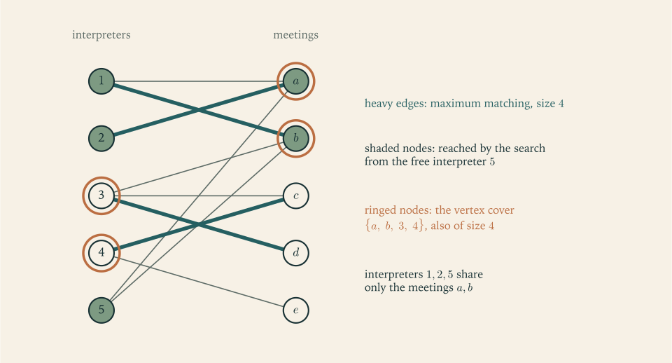
Interpreters \(1,\dots,5\) and meetings \(a,\dots,e\) have the qualifications

\[ 1:\ a,b\qquad 2:\ a\qquad 3:\ b,c,d\qquad 4:\ c,e\qquad 5:\ a,b . \]

The first coordinator’s rule gives \(1\) to \(a\) ; finds nothing for \(2\) ; gives \(3\) to \(b\) and \(4\) to \(c\) ; finds nothing for \(5\) . The matching is \(M=\{1a,\ 3b,\ 4c\}\) , of size \(3\) .

First search. Start from the free interpreter \(2\) . Its only edge leads to \(a\) , which is matched to \(1\) . From \(1\) the unmatched edge \(1b\) leads to \(b\) , matched to \(3\) . From \(3\) the unmatched edges lead to \(c\) , which is matched, and to \(d\) , which is free. The path \(2,a,1,b,3,d\) is augmenting. Exchange along it: remove \(1a\) and \(3b\) , insert \(2a\) , \(1b\) , and \(3d\) . The matching is now \(M=\{2a,\ 1b,\ 3d,\ 4c\}\) , of size \(4\) . No interpreter kept the meeting first assigned, except \(4\) .

Second search. Start from the free interpreter \(5\) . Its edges lead to \(a\) and \(b\) , matched to \(2\) and \(1\) . From \(2\) the only edge is \(2a\) itself. From \(1\) the unmatched edge leads to \(a\) , already visited. The search ends without reaching a free meeting. The set of nodes reached is \(Z=\{5,2,1,a,b\}\) .

By Theorem 4.4 the matching of size \(4\) is maximum. The stalled search also hands over the proof for the manager. Take the meetings that were reached, \(a\) and \(b\) , together with the interpreters that were not, \(3\) and \(4\) . Every edge has an endpoint in \(C=\{a,b,3,4\}\) : the edges of interpreters \(1\) , \(2\) , and \(5\) all go to \(a\) or \(b\) , and the others start at \(3\) or \(4\) . So \(C\) is a vertex cover of size \(4\) , and by Lemma 4.2 no matching has more than four edges. Put differently, interpreters \(1\) , \(2\) , and \(5\) are qualified only for meetings \(a\) and \(b\) , and three people cannot cover two meetings one each.

4.3 König’s theorem and Hall’s condition

The construction at the end of Example 4.1 works in every bipartite graph.

This is the max-flow min-cut theorem for the matching network of Section 3.5: the arcs leaving the cut \(S=\{s\}\cup Z\) are the source arcs of the nodes in \(L\setminus Z\) and the sink arcs of the nodes in \(R\cap Z\) , one arc of capacity one for each node of \(C\) . The direct proof is worth having because it shows exactly which nodes to take.

For a set \(X\) of nodes, write \(N(X)\) for the set of nodes adjacent to at least one member of \(X\) .

A set \(X\) with \(\lvert N(X)\rvert<\lvert X\rvert\) is a Hall violator. In Example 4.1 it was \(X=\{1,2,5\}\) with \(N(X)=\{a,b\}\) . Hall’s theorem says that the obvious obstruction to a complete assignment, a group that collectively has too few options, is the only obstruction.

4.4 The assignment problem and its prices

It is a minimum-cost flow problem in the sense of Definition 2.7, with a unit of supply at each row and a unit of demand at each column, and the potentials of Theorem 2.8 become a price \(p_i\) on each row and a price \(q_j\) on each column.

In the language of Continuous Optimization, the prices are a feasible solution of the dual of the relaxation, the lemma is weak duality, and tightness is complementary slackness. The differences \(c_{ij}-p_i-q_j\ge 0\) are the reduced costs. An assignment problem with reduced costs in place of costs has the same optimal assignments, since every assignment’s cost changes by the same constant; and if the reduced costs contain an assignment made entirely of zeros, that assignment is optimal.

4.5 The Hungarian method

The method keeps feasible prices and a matching in the equality graph, the bipartite graph whose edges are the tight pairs, and alternates two moves: enlarge the matching by an augmenting path when the equality graph has one, and otherwise change the prices to create new tight pairs.

Initial prices. Set \(p_i\) to the smallest cost in row \(i\) , then \(q_j\) to the smallest value of \(c_{ij}-p_i\) in column \(j\) . Every row and every column now has a zero reduced cost.

Matching step. Find a maximum matching \(M\) in the equality graph by the method of Section 4.2. If it is perfect, stop.

Price step. Otherwise, as in the proof of Theorem 4.5, let \(Z\) be the set of nodes reachable from the free rows by alternating paths in the equality graph; let \(S\) be the rows in \(Z\) and \(T\) the columns in \(Z\) . Compute

raise \(p_i\) by \(\delta\) for every \(i\in S\) , lower \(q_j\) by \(\delta\) for every \(j\in T\) , and return to the matching step.

Each search and price step costs \(O(n^2)\) operations, for a total of \(O(n^4)\) ; an implementation that updates the search instead of restarting it achieves \(O(n^3)\) . Both bounds are independent of the size of the costs.

4.6 Fractional assignments are mixtures

The relaxation of the assignment problem allows \(0\le x_{ij}\le 1\) . A nonnegative matrix whose rows and columns all sum to one is called doubly stochastic; a doubly stochastic matrix with entries \(0\) and \(1\) is a permutation matrix, which is the same thing as an assignment. Could a fractional doubly stochastic matrix be cheaper than every assignment? The Hungarian method already says no, since its prices bound the relaxation too. A structural theorem says more.

Exercises

1. In the bipartite graph with left nodes \(1,2,3,4\) , right nodes \(a,b,c,d\) , and adjacencies \(1:a,b\) ; \(2:a\) ; \(3:a,b\) ; \(4:b,c,d\) , start from the matching \(\{1a,4b\}\) and run the augmenting path algorithm, searching from the free left nodes in increasing order; report each augmenting path, the final matching, the set \(Z\) , and the vertex cover of Theorem 4.5.

   Solution

   The free left nodes are \(2\) and \(3\) .

   Search from \(2\) . The only edge of \(2\) leads to \(a\) , matched to \(1\) . From \(1\) the unmatched edge \(1b\) leads to \(b\) , matched to \(4\) . From \(4\) the unmatched edges lead to \(c\) and \(d\) , both free; take \(c\) . The augmenting path is \(2,a,1,b,4,c\) . Remove \(1a\) and \(4b\) and insert \(2a\) , \(1b\) , \(4c\) : the matching becomes \(\{2a,\ 1b,\ 4c\}\) .

   Search from \(3\) . Its edges lead to \(a\) , matched to \(2\) , and to \(b\) , matched to \(1\) . Node \(2\) has no other edge; node \(1\) leads back to \(a\) . No free right node is reached. The set of reached nodes is \(Z=\{3,2,1,a,b\}\) .

   By Theorem 4.4 the matching \(\{2a,1b,4c\}\) of size \(3\) is maximum. The cover of Theorem 4.5 is \(C=(L\setminus Z)\cup(R\cap Z)=\{4\}\cup\{a,b\}\) . Check: the edges of nodes \(1\) , \(2\) , \(3\) all end in \(a\) or \(b\) , and the edges of node \(4\) are covered by \(4\) . The cover has three nodes and the matching three edges, so both are optimal by Lemma 4.2. Each matching edge has exactly one endpoint in \(C\) : \(2a\) and \(1b\) at their right ends, \(4c\) at its left end.

2. For the graph of Exercise 1, exhibit a Hall violator, and state how many left nodes can be matched according to the formula \(\lvert L\rvert-\max_X(\lvert X\rvert-\lvert N(X)\rvert)\) , checking it against your matching.

   Answer

   \(X=\{1,2,3\}\) has \(N(X)=\{a,b\}\) , so \(\lvert X\rvert-\lvert N(X)\rvert=1\) . No set has a larger deficiency, since a matching of size \(3\) exists, and \(4-1=3\) agrees with the matching found in Exercise 4.1.

3. Prove that if \(M\) and \(M'\) are matchings in any graph, every connected piece of the graph formed by the edges in exactly one of them is a path or a cycle of even length, and explain where your proof uses the fact that both are matchings.

   Solution

   Let \(H\) be the graph formed by the edges lying in exactly one of \(M\) and \(M'\) . A node is an endpoint of at most one edge of \(M\) and at most one edge of \(M'\) , because each is a matching; so every node has degree at most \(2\) in \(H\) . A connected graph in which every degree is at most \(2\) is a path or a cycle: follow edges from any node in both directions; at each node there is at most one way to continue, so the walk either stops at nodes of degree one, giving a path, or returns to its start, giving a cycle.

   At a node of degree \(2\) in \(H\) , one of the two edges belongs to \(M\) and the other to \(M'\) , since two edges of the same matching cannot meet. So along each path or cycle the edges alternate between \(M\) and \(M'\) . A cycle whose edges alternate between two classes has an even number of edges, since otherwise two edges of the same class would meet at the node where the count wraps around.

   The hypothesis that both sets are matchings was used twice: to bound degrees by two, and to force alternation at every node of degree two. Without it, for instance for two arbitrary edge sets, pieces of \(H\) can branch.

4. Five committees have the member lists \(\{u,v\}\) , \(\{v,w\}\) , \(\{u,w\}\) , \(\{u,v,w\}\) , and \(\{w,x,y\}\) . Decide whether each committee can be given a chairperson from among its members so that no person chairs two committees, proving your answer with a matching or a Hall violator.

   Solution

   No. Consider the first four committees, \(\{u,v\}\) , \(\{v,w\}\) , \(\{u,w\}\) , and \(\{u,v,w\}\) . Every member of each of them belongs to \(\{u,v,w\}\) . In the bipartite graph with committees on the left and people on the right, where a committee is joined to its members, this set \(X\) of four committees has \(N(X)=\{u,v,w\}\) , so \(\lvert N(X)\rvert=3<4=\lvert X\rvert\) . That is a Hall violator, and by Theorem 4.6 no matching covers all five committees: four committees cannot have four different chairs drawn from three people.

   The best possible is four committees with distinct chairs, for example \(u\) for the first, \(v\) for the second, \(w\) for the third, and \(x\) for the fifth, leaving the fourth without a chair of its own. This matching has size \(4\) , and the cover consisting of \(u\) , \(v\) , \(w\) , and the fifth committee has size \(4\) , which confirms by Lemma 4.2 that four is the maximum.

5. Prove by induction on \(k\) that the edge set of a \(k\) -regular bipartite graph is the union of \(k\) pairwise disjoint perfect matchings, and deduce that \(n\) teams on each of two sides, each pair meeting once, can be scheduled in \(n\) rounds.

   Solution

   Claim. The edges of a \(k\) -regular bipartite graph are the union of \(k\) pairwise disjoint perfect matchings.

   For \(k=1\) every node has exactly one edge, so the edge set is itself a perfect matching. Suppose the claim holds for \(k-1\ge 1\) and let \(G\) be \(k\) -regular. By Corollary 4.7, \(G\) has a perfect matching \(M_k\) . Remove its edges. Every node lost exactly one edge, since a perfect matching meets every node once, so the remaining graph is \((k-1)\) -regular and bipartite on the same node sets. By the induction hypothesis its edges are the union of disjoint perfect matchings \(M_1,\dots,M_{k-1}\) , none of which contains an edge of \(M_k\) . Together \(M_1,\dots,M_k\) are disjoint and exhaust the edges of \(G\) .

   Application. Let the two sides be the two groups of \(n\) teams, with an edge for every pair consisting of one team from each side. Every node has degree \(n\) , so the graph is \(n\) -regular and its edges split into \(n\) perfect matchings. Each perfect matching is a round in which every team plays exactly once, and every pair meets in exactly one round. So \(n\) rounds suffice, and fewer are impossible because each team has \(n\) games and plays at most one per round.

6. For the cycle on five nodes find the maximum size of a matching and the minimum size of a vertex cover, and identify the step in the proof of Theorem 4.5 that has no meaning when the graph is not bipartite.

   Answer

   The maximum matching has \(2\) edges and the minimum vertex cover has \(3\) nodes: two nodes cover at most four of the five edges. The proof of Theorem 4.5 begins by fixing sides \(L\) and \(R\) and searching from \(L\) along non-matching edges and back along matching edges; an odd cycle has no such sides, so the set \(Z\) and the cover \((L\setminus Z)\cup(R\cap Z)\) are not defined.

7. Apply the Hungarian method to the cost matrix with rows \((7,2,8)\) , \((9,1,3)\) , \((5,5,4)\) : give the initial prices and reduced costs, the sets \(S\) and \(T\) and the value of \(\delta\) in the price step, and the final assignment with prices certifying it.

   Solution

   Initial prices. Row minima: \(p=(2,1,4)\) . After subtracting, the rows are \((5,0,6)\) , \((8,0,2)\) , \((1,1,0)\) , with column minima \(1,0,0\) , so \(q=(1,0,0)\) and the price total is \(8\) . The reduced costs are

   \[ \begin{pmatrix}4&0&6\\7&0&2\\0&1&0\end{pmatrix}. \]

   The tight pairs are \((1,2)\) , \((2,2)\) , \((3,1)\) , \((3,3)\) . A maximum matching in the equality graph is \(\{(1,2),(3,1)\}\) ; row \(2\) is free.

   Price step. From row \(2\) the search reaches column \(2\) and its partner row \(1\) , which has no other tight pair. So \(S=\{1,2\}\) and \(T=\{2\}\) . The reduced costs in rows \(1,2\) and columns \(1,3\) are \(4,6\) and \(7,2\) , so \(\delta=2\) , attained at \((2,3)\) . The new prices are \(p=(4,3,4)\) and \(q=(1,-2,0)\) , with total \(10\) , and the reduced costs are

   \[ \begin{pmatrix}2&0&4\\5&0&0\\0&3&0\end{pmatrix}. \]

   Augmentation. Row \(2\) now reaches the free column \(3\) directly. The perfect matching is \((1,2)\) , \((2,3)\) , \((3,1)\) , with cost \(2+3+5=10\) , equal to the price total \(4+3+4+1-2+0=10\) . By Lemma 4.9 it is optimal.

8. For the cost matrix with rows \((8,8,1)\) , \((3,5,9)\) , \((7,8,4)\) , verify with Lemma 4.9 that the assignment of row 1 to column 3, row 2 to column 1, and row 3 to column 2 is optimal, using the prices \(p=(3,3,6)\) and \(q=(0,2,-2)\) .

   Solution

   First check feasibility of the prices, that is, \(p_i+q_j\le c_{ij}\) for all nine pairs. The sums \(p_i+q_j\) form the matrix with rows \((3,5,1)\) , \((3,5,1)\) , \((6,8,4)\) . Compare with the costs \((8,8,1)\) , \((3,5,9)\) , \((7,8,4)\) : every entry of the first is at most the corresponding entry of the second. The reduced costs are

   \[ \begin{pmatrix}5&3&0\\0&0&8\\1&0&0\end{pmatrix}, \]

   all nonnegative. So by Lemma 4.9 every assignment costs at least \(p_1+p_2+p_3+q_1+q_2+q_3=12+0=12\) .

   The proposed assignment uses the pairs \((1,3)\) , \((2,1)\) , \((3,2)\) , whose reduced costs are \(0\) , \(0\) , \(0\) : all tight. Its cost is \(1+3+8=12\) , equal to the bound, so it is optimal. Notice that it uses the entry \(8\) , the largest in its row, and that the tempting diagonal entry \(c_{33}=4\) , although tight, is not used; an optimal assignment is a matching among tight pairs, and not every tight pair need appear in it.

9. A firm wants the assignment of maximum total profit for an \(n\times n\) profit matrix. Show how to convert the problem into a minimization problem with nonnegative costs to which the Hungarian method applies, and carry out the conversion for the matrix of Example 4.3 regarded as profits, giving the new matrix.

   Answer

   Let \(K\) be the largest profit and put \(c_{ij}=K-\text{profit}_{ij}\ge 0\) . Every assignment has cost \(nK\) minus its profit, so minimum cost is maximum profit. For the matrix of Example 4.3, \(K=9\) and the cost matrix has rows \((1,7,0,6)\) , \((1,6,2,0)\) , \((6,3,7,6)\) , \((1,2,0,4)\) .

10. Three workers must be assigned to three of four tasks, one task being left undone, at minimum cost. Explain how to model this as a square assignment problem with a fourth, dummy worker, and say what the dummy’s assigned task represents.

    Hint

    Add a fourth row whose costs are all zero, or all equal to any constant. In an optimal assignment of the \(4\times 4\) problem the three real workers take three distinct tasks at minimum total cost, and the task assigned to the dummy is the one left undone. A constant row does not affect which assignments are optimal; compare Exercise 4.12.

11. Explain what is wrong with this claim, using Example 4.3: “After subtracting row minima and then column minima, pick the zero in each row; if two rows pick the same column, give that column to the row whose next-smallest reduced cost is larger.”

    Solution

    In Example 4.3 the reduced costs after the initial prices are

    \[ \begin{pmatrix}5&0&7&1\\4&0&4&6\\0&4&0&1\\2&2&4&0\end{pmatrix}. \]

    Rows \(1\) and \(2\) both pick column \(2\) . Their next-smallest reduced costs are \(1\) and \(4\) , so the rule gives column \(2\) to row \(2\) and sends row \(1\) to its next choice, column \(4\) . But row \(4\) has already picked column \(4\) , its only zero. The rule must be applied again, between rows \(1\) and \(4\) , whose next-smallest reduced costs are \(5\) and \(2\) ; row \(1\) keeps column \(4\) and row \(4\) moves to a column with reduced cost \(2\) . If it moves to column \(1\) , row \(3\) takes column \(3\) , and the result happens to be the optimal assignment; if it moves to column \(2\) it collides again.

    So the rule is not a well-defined algorithm, and when it succeeds it does so without proof. The underlying error is treating reduced costs as if conflicts could be resolved one pair of rows at a time. A conflict in one column propagates along an alternating path, here through columns \(2\) , \(4\) , and \(1\) , and it is resolved by a price step that changes many reduced costs at once and keeps a certificate. The Hungarian method is what the rule is groping towards.

12. Prove that adding a constant \(\alpha\) to every entry of one row of a cost matrix changes the cost of every assignment by \(\alpha\) and so leaves the set of optimal assignments unchanged, and relate this to Exercise 2.7 on potentials.

    Hint

    Every assignment uses exactly one entry of the altered row, so its cost changes by exactly \(\alpha\) , and the ordering of assignments by cost is unchanged. This is the potential shift of Exercise 2.7 with \(\pi\) changed at a single node: all paths between fixed endpoints there, and all assignments here, change by the same constant.

13. Build the unit-capacity flow network of Section 3.5 for the graph of Example 4.1, state the maximum flow and a minimum cut, and show how the cut’s capacity-one arcs correspond to the cover \(\{a,b,3,4\}\) .

    Hint

    Arcs: \(s\) to each interpreter, capacity \(1\) ; interpreter to each meeting it is qualified for, capacity \(1\) ; each meeting to \(t\) , capacity \(1\) . The maximum flow is \(4\) . Take \(S=\{s\}\cup Z=\{s,1,2,5,a,b\}\) . The arcs leaving \(S\) are \(s\) to \(3\) , \(s\) to \(4\) , \(a\) to \(t\) , and \(b\) to \(t\) ; no arc from \(1\) , \(2\) , or \(5\) leaves \(S\) .

14. Write the doubly stochastic matrix with rows \((\tfrac13,\tfrac23,0)\) , \((\tfrac23,0,\tfrac13)\) , \((0,\tfrac13,\tfrac23)\) as a convex combination of permutation matrices by the procedure of Theorem 4.11.

    Answer

    The permutation using positions \((1,2)\) , \((2,1)\) , \((3,3)\) has entries \(\tfrac23,\tfrac23,\tfrac23\) ; subtracting \(\tfrac23\) of it leaves \(\tfrac13\) at \((1,1)\) , \((2,3)\) , \((3,2)\) . So the matrix is \(\tfrac23\) of the permutation matrix that swaps the first two and fixes the third, plus \(\tfrac13\) of the one that fixes the first and swaps the other two.

15. In the bottleneck assignment problem the cost of an assignment is its largest entry. Explain how to solve it with a bisection over thresholds as in Proposition 1.6 and a bipartite matching computation for each threshold, and find the bottleneck optimum for the matrix of Example 4.3.

    Solution

    For a threshold \(\theta\) , an assignment with largest entry at most \(\theta\) exists exactly when the bipartite graph containing the pairs with \(c_{ij}\le\theta\) has a perfect matching. That is a decision question answered by one matching computation, and the answer is monotone: yes for every \(\theta\) above the optimum, no below. The optimum is one of the \(n^2\) entries, so sorting them and bisecting over the sorted list as in Proposition 1.6 needs at most \(\lceil\log_2 n^2\rceil\) matching computations.

    For the matrix of Example 4.3 the distinct entries are \(2,3,5,6,7,8,9\) . With \(\theta=6\) the allowed pairs are: row \(1\) with columns \(2,4\) ; row \(2\) with column \(2\) ; row \(3\) with all columns; row \(4\) with column \(4\) . Rows \(1\) , \(2\) , \(4\) have only columns \(2\) and \(4\) between them, a Hall violator, so there is no perfect matching. With \(\theta=7\) row \(2\) gains column \(3\) and row \(4\) gains column \(2\) , and \((1,2)\) , \((2,3)\) , \((3,1)\) , \((4,4)\) is a perfect matching with entries \(2,7,3,5\) .

    The bottleneck optimum is \(7\) . That assignment has total \(17\) , while the minimum-total assignment of Example 4.3 has total \(16\) and largest entry \(8\) : the two objectives disagree.

16. Prove that a bipartite graph with \(m\) edges in which every node has degree at most \(\Delta\) has a matching with at least \(m/\Delta\) edges.

    Solution

    Let \(C\) be a minimum vertex cover. Each node of \(C\) covers at most \(\Delta\) edges, namely those incident with it, and every one of the \(m\) edges is covered by at least one node of \(C\) . Hence \(m\le\Delta\lvert C\rvert\) , that is, \(\lvert C\rvert\ge m/\Delta\) .

    By Theorem 4.5 the graph, being bipartite, has a matching \(M\) with \(\lvert M\rvert=\lvert C\rvert\) . Therefore \(\lvert M\rvert\ge m/\Delta\) .

    The argument shows the pattern of use of a min-max theorem: to prove that a large matching exists, prove that every cover is large, which is a counting statement about covers and needs no construction of a matching. Without bipartiteness the argument gives nothing, since König’s equality may fail; the statement itself is weaker in general graphs. In a triangle, \(m/\Delta=3/2\) and the maximum matching has size \(1\) .

17. In the Hungarian method, suppose the costs are integers. Using only the fact that the price total increases by a positive integer in every price step and never exceeds the optimal cost, give a bound on the number of price steps, and explain why this bound is weaker than the one in Theorem 4.10 in the sense of Chapter 1.

    Hint

    The price total is an integer that starts at some value \(B_0\ge n\min_{i,j}c_{ij}\) , never exceeds the optimal cost, which is at most \(n\max_{i,j}c_{ij}\) , and rises by at least one per price step. So there are at most \(n(\max c-\min c)\) price steps. That bound depends on the magnitudes of the costs, so it is pseudo-polynomial; the bound \(n^2\) of Theorem 4.10 depends on \(n\) alone.

18. A student applies Corollary 4.12 to the triangle graph and concludes that its fractional matching relaxation has an integral optimum. Explain which hypothesis of Theorem 4.11 has no counterpart for the triangle, and give the fractional optimum and the integral optimum for unit edge weights.

    Answer

    Theorem 4.11 is about matrices whose rows and columns form the two sides of a bipartite graph, and its proof applies Hall’s theorem to that graph. The triangle has no two sides. With unit weights the fractional optimum puts \(\tfrac12\) on each edge, total \(\tfrac32\) ; the integral optimum is a single edge, total \(1\) .