A charter aircraft carries two kinds of pallet. A pallet of the first kind earns a profit of 5, occupies one floor position, and weighs 3 tonnes. A pallet of the second kind earns 4, occupies two floor positions, and weighs 2 tonnes. The aircraft has 8 floor positions and a payload limit of 11 tonnes. How many pallets of each kind should it carry?

If fractions of a pallet were allowed, this would be a linear program, and the methods of Continuous Optimization would finish it at once: carry \(1.5\) pallets of the first kind and \(3.25\) of the second, for a profit of \(20.5\) . Pallets do not come in quarters. The obvious repair, rounding, fails here in an instructive way, and the best whole-number plan turns out to sit nowhere near the fractional one. This chapter sets up the language for such problems, shows how yes-or-no decisions are written as algebra, and explains what it means to call one problem easy and another hard. The cargo problem returns in Chapters 5, 7, and 8, where it is solved three more times by three different methods.

1.1 Optimizing over a finite set

The word implicitly carries the whole subject. A finite set always has a best element, so existence of an optimum, which takes real work for continuous problems, is free here. What is not free is finding it. The data of an instance is short, a few numbers or a graph, while the set \(\mathcal F\) it describes is typically astronomically large: a graph on \(n\) nodes can have \(n^{n-2}\) spanning trees, an assignment of \(n\) workers to \(n\) jobs can be made in \(n!\) ways, and \(n\) yes-or-no decisions can be made in \(2^n\) ways. Listing \(\mathcal F\) is not an algorithm one can use.

Most problems in this book can be written in one common algebraic form.

A minimization problem fits the definition after the objective is negated, and an equality constraint is two inequalities. The relaxation is a linear program in the sense of Continuous Optimization, so it can be solved efficiently, and it bounds the integer problem. That bound is one half of a pair of inequalities on which every exact method in this book rests.

A feasible solution proves a lower bound on \(z^\star\) ; a relaxation proves an upper bound. When the two meet, optimality has been proved, and the pair is a certificate that anyone can check without repeating the search. When they do not meet, their difference is a guaranteed limit on how far the solution in hand is from optimal.

Example 1.1: The cargo problem by enumeration

Let \(x_1\) and \(x_2\) be the numbers of pallets of the two kinds. The cargo problem is

\[ \begin{aligned} \text{maximize}\quad & 5x_1+4x_2\\ \text{subject to}\quad & x_1+2x_2\le 8,\\ & 3x_1+2x_2\le 11,\\ & x_1,x_2\ge 0\ \text{and integer}. \end{aligned} \]

The first constraint counts floor positions and the second counts tonnes. The relaxation is a linear program in two variables whose feasible region is a quadrilateral with vertices \((0,0)\) , \((11/3,0)\) , \((3/2,13/4)\) , and \((0,4)\) . The objective takes the values \(0\) , \(55/3\) , \(41/2\) , and \(16\) there, so the relaxation optimum is \(x_{LP}=(3/2,13/4)\) with \(z_{LP}=41/2\) , where both constraints are active.

Now round. The four integer points surrounding \(x_{LP}\) are \((1,3)\) , \((2,3)\) , \((1,4)\) , and \((2,4)\) . The point \((2,3)\) weighs \(3\cdot 2+2\cdot 3=12\) tonnes, which exceeds \(11\) . The points \((1,4)\) and \((2,4)\) need \(9\) and \(10\) floor positions, which exceed \(8\) . Only \((1,3)\) is feasible, with profit \(5+12=17\) .

Is \(17\) the answer? The feasible integer points can be listed column by column. For \(x_1=0\) the constraints allow \(x_2\le 4\) ; for \(x_1=1\) , \(x_2\le 3\) ; for \(x_1=2\) , \(x_2\le 2\) ; for \(x_1=3\) , \(x_2\le 1\) ; and \(x_1=4\) already weighs \(12\) tonnes. That makes \(5+4+3+2=14\) feasible points. The best in each column is \((0,4)\) with profit \(16\) , \((1,3)\) with \(17\) , \((2,2)\) with \(18\) , and \((3,1)\) with \(19\) . So the integer optimum is \(x^\star=(3,1)\) with \(z^\star=19\) , two units better than the rounded plan and at a quite different mix of pallets.

Proposition 1.3 brackets the answer without the enumeration: any feasible plan gives a lower bound and the relaxation gives \(z^\star\le\lfloor 41/2\rfloor=20\) . With \((1,3)\) in hand one knows \(17\le z^\star\le 20\) ; with \((3,1)\) in hand, \(19\le z^\star\le 20\) . Closing the last gap, proving that \(20\) is not attainable, is the business of Chapters 7 and 8.

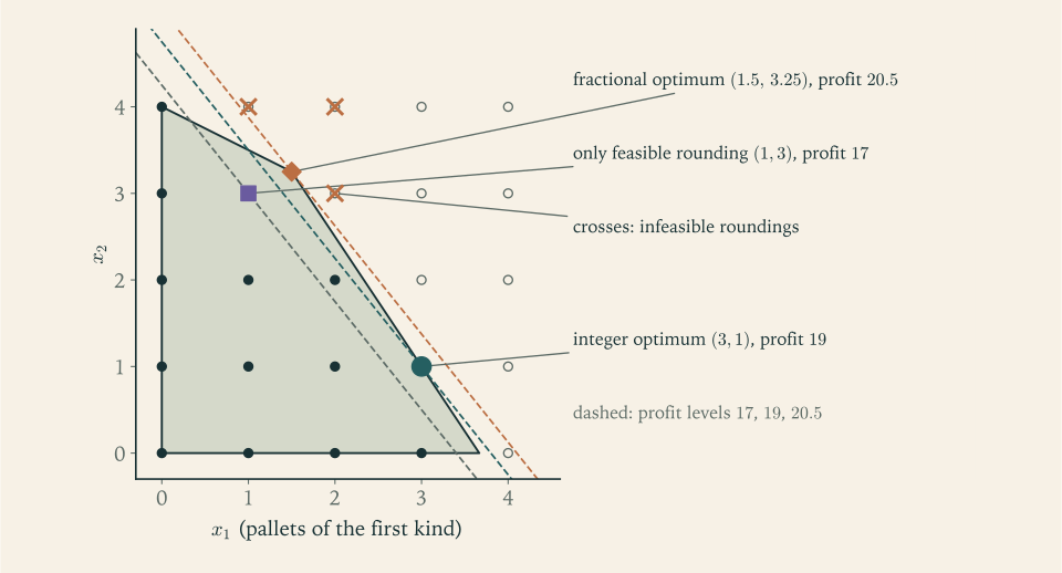
Common mistake. Solving the relaxation and rounding its solution to the nearest integers. In Example 1.1 the nearest integer point \((2,3)\) is infeasible, the only feasible neighbour is not optimal, and the true optimum is not a neighbour at all. Rounding can be made rigorous for particular problems, and Chapter 10 does so with a proof each time; as a general recipe it produces neither feasibility nor optimality. What the relaxation always gives is the bound \(z_{LP}\) .

1.2 Writing decisions as algebra

Binary variables turn logical statements into linear inequalities. Let \(x_i\in\{0,1\}\) record whether option \(i\) is chosen. The statement “at most one of options 3 and 4” is \(x_3+x_4\le 1\) . “Option 2 may be chosen only if option 1 is” is \(x_2\le x_1\) . “At least two of the options in a set \(S\) ” is \(x(S)\ge 2\) . “Options 3 and 5 exclude each other” is \(x_3+x_5\le 1\) . Each translation is checked the same way: list the 0–1 combinations the sentence forbids and confirm that the inequality cuts off exactly those.

A binary variable can also switch a continuous quantity on and off. Suppose \(y\ge 0\) is a production quantity that can be positive only if a fixed cost is paid, and suppose \(y\) can never exceed a known number \(M\) . With \(x\in\{0,1\}\) recording whether the cost is paid, the constraint

forces \(y\) to be zero when \(x\) is zero and imposes nothing beyond \(y\le M\) when \(x\) is one. The total cost \(fx+cy\) then charges the fixed amount \(f\) exactly when it must. The same device expresses a choice between two constraints. To require that at least one of \(a^{\top}y\le\beta\) and \(d^{\top}y\le\gamma\) holds, introduce \(x\in\{0,1\}\) and write \(a^{\top}y\le\beta+Mx\) and \(d^{\top}y\le\gamma+M(1-x)\) , where \(M\) is large enough that adding it makes either constraint vacuous on the region of interest. The constant \(M\) must be a valid bound, and Chapter 5 explains why it should also be as small as possible.

1.3 How large is an instance?

To compare algorithms we count their elementary steps as a function of the size of the input. The size is not the number of data items and not their magnitude; it is the amount of writing needed to state the instance.

A number of magnitude \(W\) has encoding length about \(\log_2 W\) , so \(W\) itself is exponential in the space it occupies. An algorithm whose running time is proportional to \(W\) therefore takes time exponential in the input size, even though the formula for its running time looks innocent. Chapter 9 develops exactly such an algorithm for the knapsack problem, with a table of \(n(W+1)\) entries, and the next example measures what that means.

1.4 From yes-or-no questions to optimal solutions

Complexity theory is built on decision problems, whose answer is yes or no. Every optimization problem has a decision version: given an instance and a threshold \(k\) , is there a feasible solution with objective value at least \(k\) ? Nothing is lost by this restriction, because an algorithm for the decision version can be turned into one for the optimization version with few extra calls.

The number of calls is the encoding length of the range, so it is polynomial in the input size whenever \(U\) and \(\ell\) are computed from the data by sums and products, as they are for integer programs with bounded variables. For binary programs the optimal solution itself can then be recovered by fixing variables one at a time: ask whether value \(z^\star\) is still achievable with \(x_1=1\) ; if so fix it, if not fix \(x_1=0\) ; continue with \(x_2\) . That costs \(n\) further calls.

1.5 Certificates, the classes P and NP, and reductions

Membership in NP says that yes-answers can be checked quickly once someone supplies the evidence; it says nothing about how to find the evidence. For the decision version of a binary program the certificate is the solution \(x\) itself: it has \(n\) bits, and checking \(Ax\le b\) and \(c^{\top}x\ge k\) takes one pass over the data. Every problem in P is in NP, with an empty certificate. Whether the two classes are equal is the central open problem of the subject, and this book, like all practical work, proceeds on the assumption that they are not.

A reduction from \(\Pi_1\) to \(\Pi_2\) shows that \(\Pi_2\) is at least as hard as \(\Pi_1\) : a polynomial algorithm for \(\Pi_2\) , composed with the transformation, would be a polynomial algorithm for \(\Pi_1\) . Reductions compose, so if an NP-hard problem reduces to \(\Pi_2\) then \(\Pi_2\) is NP-hard.

The simplest reductions are relabelings. In an undirected graph, a set of nodes is independent if no edge joins two of its members, a vertex cover if every edge has at least one endpoint in it, and a clique if every two of its members are joined by an edge.

1.6 Three responses to hardness

The feasible set of the assignment problem has \(n!\) elements and the problem is solved in \(O(n^3)\) steps. The feasible set of a knapsack problem has at most \(2^n\) elements and no polynomial algorithm is known. The size of \(\mathcal F\) does not decide difficulty; structure does. The rest of this book is organized around three responses to that fact.

The first response is to exploit structure. Shortest paths, maximum flows, and bipartite matchings, the subjects of Chapters 2 to 4, have optimality conditions that can be checked locally and algorithms that improve a solution until the conditions hold. Chapter 6 explains through polyhedral geometry why these problems behave so well: their linear programming relaxations have only integer vertices, so the upper bound of Proposition 1.3 is always attained.

The second response is to search with bounds. When the relaxation does not have integer vertices, as in the cargo problem, Proposition 1.3 still supplies an upper bound for any part of the feasible set. Chapter 5 studies how the choice of formulation changes that bound, Chapter 7 uses it to discard most of an enumeration tree, and Chapter 8 tightens it by adding inequalities that every integer solution satisfies and the fractional optimum does not.

The third response is to give up exactness in a controlled way. Chapter 9 solves the knapsack problem exactly in pseudo-polynomial time and then, by rounding the data, to within any chosen relative error in polynomial time. Chapter 10 treats algorithms that carry a proven worst-case ratio to the optimum, and decomposition methods whose bounds are sharper than those of the plain relaxation. In every case the answer comes with evidence: an exact method delivers a matching pair of bounds, an approximate one delivers a gap.

Which response a problem needs is not always visible from its statement. Finding a shortest route through a network is easy and finding a longest route without repeated nodes is NP-hard. Matching workers to jobs is easy and matching them in triples is NP-hard. Part of what the following chapters teach is how to recognize the easy structures when they are present, and how to see them hidden inside hard problems as relaxations.

Exercises

1. A city must choose which of six candidate sites \(1,\dots,6\) receive a clinic. Write linear constraints in binary variables \(x_1,\dots,x_6\) for each rule: (a) exactly three clinics are built; (b) sites 1 and 2 are not both used; (c) if site 3 is used then site 4 must be; (d) site 5 is used only if at least one of sites 1 and 6 is; (e) at least one of sites 2, 4, 6 is left unused.

   Answer

   (a) \(x_1+x_2+x_3+x_4+x_5+x_6=3\) . (b) \(x_1+x_2\le 1\) . (c) \(x_3\le x_4\) . (d) \(x_5\le x_1+x_6\) . (e) \(x_2+x_4+x_6\le 2\) . For (d), check the forbidden case: \(x_5=1\) with \(x_1=x_6=0\) gives \(1\le 0\) , which is violated, and every other combination satisfies the inequality.

2. For the integer program that maximizes \(x_2\) subject to \(-2x_1+2x_2\le 1\) , \(2x_1+2x_2\le 7\) , and \(x_1,x_2\ge 0\) integer, find the relaxation optimum, show that every integer point obtained by rounding its coordinates up or down is infeasible, and find \(z^\star\) and all optimal integer solutions.

   Solution

   Adding the two constraints gives \(4x_2\le 8\) , so every point of the relaxation has \(x_2\le 2\) , and \(x_2=2\) forces both constraints to be active: \(-2x_1+4=1\) and \(2x_1+4=7\) , so \(x_1=3/2\) . The relaxation optimum is \(x_{LP}=(3/2,2)\) with \(z_{LP}=2\) .

   The second coordinate is already an integer, so rounding means replacing \(x_1\) by \(1\) or \(2\) . At \((1,2)\) the first constraint reads \(-2+4=2>1\) . At \((2,2)\) the second reads \(4+4=8>7\) . Both roundings are infeasible.

   For integer points, the first constraint \(-2x_1+2x_2\le 1\) has an even left side, so it is equivalent to \(-2x_1+2x_2\le 0\) , that is \(x_2\le x_1\) . The second has an even left side as well, so it is equivalent to \(2x_1+2x_2\le 6\) , that is \(x_1+x_2\le 3\) . Adding, \(2x_2\le 3\) , so \(x_2\le 1\) . The value \(x_2=1\) needs \(1\le x_1\le 2\) . Hence \(z^\star=1\) , attained at \((1,1)\) and \((2,1)\) . The relaxation bound \(\lfloor z_{LP}\rfloor=2\) is not attained, and the integer optima are not roundings of the fractional one. The parity argument used here is the rounding idea that Chapter 8 turns into a general method.

3. Compute the encoding length \(\langle k\rangle\) of each of \(5\) , \(64\) , \(1000\) , and \(2^{20}-1\) , and give the total number of bits needed to write the capacity and the ten item weights of a knapsack instance in which every one of those eleven numbers lies between \(2^{15}\) and \(2^{16}-1\) .

   Answer

   \(\langle 5\rangle=3\) , \(\langle 64\rangle=7\) , \(\langle 1000\rangle=10\) , and \(\langle 2^{20}-1\rangle=20\) . A number between \(2^{15}\) and \(2^{16}-1\) has exactly \(16\) binary digits, so the eleven numbers take \(11\cdot 16=176\) bits.

4. Classify each running time as polynomial, pseudo-polynomial but not polynomial, or exponential in \(n\) , for an instance with \(n\) numbers of which the largest is \(W\) , and justify each answer in terms of encoding length: (a) \(n^3\) ; (b) \(nW\) ; (c) \(n\log_2 W\) ; (d) \(2^n\) ; (e) \(n^2\sqrt W\) ; (f) \(n(\log_2 W)^3\) .

   Hint

   Write \(L\) for the encoding length; then \(n\le L\) and \(\log_2 W\le L\) , while \(W\) can be as large as about \(2^{L}\) . (a), (c), and (f) are bounded by polynomials in \(L\) . (b) and (e) are polynomial in \(n\) and \(W\) but not in \(L\) : \(\sqrt W\) can be \(2^{L/2}\) . (d) is exponential in \(n\) whatever the numbers are.

5. Consider knapsack instances restricted so that the capacity satisfies \(W\le n^2\) . Prove that on this restricted family an algorithm running in \(O(nW)\) steps is polynomial, and explain why this does not contradict the NP-hardness of the knapsack problem.

   Solution

   Every instance contains at least the \(n\) item weights and profits, each occupying at least one bit, so the encoding length satisfies \(L\ge n\) . On the restricted family \(W\le n^2\) , so the number of steps is at most a constant times \(nW\le n^3\le L^3\) . That is a polynomial bound in the encoding length, so the algorithm is polynomial on this family.

   There is no contradiction with NP-hardness, because NP-hardness is a statement about the whole problem, including instances whose capacity is enormous compared with \(n\) . The reduction from subset sum in Proposition 1.11 produces knapsack instances whose weights are the given integers, and those may have hundreds of digits with \(n\) small; such instances lie outside the restricted family. A problem can be NP-hard and still have large families of instances that are easy. What the restriction shows is that the difficulty of knapsack lives in the size of its numbers, which is the meaning of weak NP-hardness.

6. A binary program in which \(x=0\) is feasible has \(40\) variables and objective coefficients that are integers between \(0\) and \(1000\) . Give the best bounds \(\ell\) and \(U\) you can state without solving anything, the number of oracle calls Proposition 1.6 needs to find \(z^\star\) , and the number of further calls needed to recover an optimal solution by fixing variables.

   Answer

   \(\ell=0\) , attained by \(x=0\) , and \(U=40\cdot 1000=40000\) . There are \(40001\) candidate values and \(2^{15}=32768<40001\le 65536=2^{16}\) , so \(16\) oracle calls find \(z^\star\) . Fixing the variables one at a time takes at most \(40\) more.

7. Carry out the variable-fixing procedure described after Proposition 1.6 on Example 1.2: knowing that \(z^\star=20\) , decide for each of \(x_1,\dots,x_5\) in turn whether value \(20\) remains achievable with that variable set to one given the earlier decisions, and report the solution you obtain.

   Solution

   The oracle question at each step is: with the variables already fixed, and the current variable set to one, is there a feasible completion of value at least \(20\) ?

   Set \(x_1=1\) . The selection \((1,1,0,1,0)\) has value \(20\) , so the answer is yes; fix \(x_1=1\) . Set \(x_2=1\) . The same selection shows yes; fix \(x_2=1\) . Set \(x_3=1\) . Projects 1, 2, 3 cost \(5+3+4=12>11\) , so no feasible completion exists at all; the answer is no and \(x_3=0\) . Set \(x_4=1\) . Projects 1, 2, 4 cost \(10\) and are worth \(20\) , and the rule on projects 3 and 4 holds because \(x_3=0\) ; yes, fix \(x_4=1\) . Set \(x_5=1\) . Projects 1, 2, 4, 5 cost \(16>11\) ; no, so \(x_5=0\) .

   The procedure returns \(x=(1,1,0,1,0)\) after five calls, which is the optimal selection of Example 1.2. Each answer of “yes” was justified by a completion; each “no” here could be justified by the budget alone, which is a lucky feature of this instance and not of the method.

8. Model the following with one binary variable and a constant \(M\) , and state the smallest valid \(M\) : a machine either stays idle or produces a quantity \(y\) between \(20\) and \(75\) units, at a fixed cost of \(300\) plus \(4\) per unit.

   Answer

   With \(x\in\{0,1\}\) : \(20x\le y\le 75x\) and cost \(300x+4y\) . The smallest valid constant in \(y\le Mx\) is \(M=75\) , the largest quantity the machine can produce. If \(x=0\) then \(y=0\) and the cost is \(0\) ; if \(x=1\) then \(20\le y\le 75\) .

9. A continuous variable \(y\) with \(0\le y\le 10\) must satisfy at least one of \(y\le 3\) and \(y\ge 7\) . Write this with one binary variable, giving explicit constants, and verify your formulation by listing the values of \(y\) allowed for each value of the binary variable.

   Solution

   Let \(x=0\) select the alternative \(y\le 3\) and \(x=1\) select \(y\ge 7\) . Because \(0\le y\le 10\) throughout, the constraint \(y\le 3\) is switched off by adding \(7\) to its right side, and the constraint \(y\ge 7\) is switched off by subtracting \(7\) from its right side:

   \[ y\le 3+7x,\qquad y\ge 7x,\qquad 0\le y\le 10,\qquad x\in\{0,1\}. \]

   For \(x=0\) the constraints read \(y\le 3\) and \(y\ge 0\) , so \(0\le y\le 3\) . For \(x=1\) they read \(y\le 10\) and \(y\ge 7\) , so \(7\le y\le 10\) . The union of the two cases is exactly the required set, and the open interval between \(3\) and \(7\) is excluded for both values of \(x\) . The constants are the smallest that work: with \(y\le 3+Mx\) and \(M<7\) the case \(x=1\) would cut off values of \(y\) up to \(10\) that should be allowed.

10. Prove that if \(\Pi_1\) reduces to \(\Pi_2\) and \(\Pi_2\) reduces to \(\Pi_3\) then \(\Pi_1\) reduces to \(\Pi_3\) , taking care to explain why the composed transformation still runs in polynomial time.

    Solution

    Let \(T_1\) transform instances of \(\Pi_1\) into instances of \(\Pi_2\) in at most \(p_1(L)\) steps on inputs of length \(L\) , and let \(T_2\) transform instances of \(\Pi_2\) into instances of \(\Pi_3\) in at most \(p_2(L)\) steps, with \(p_1,p_2\) polynomials that may be taken nondecreasing. Define \(T(I)=T_2(T_1(I))\) .

    Correctness. \(I\) is a yes-instance of \(\Pi_1\) exactly when \(T_1(I)\) is a yes-instance of \(\Pi_2\) , which holds exactly when \(T_2(T_1(I))\) is a yes-instance of \(\Pi_3\) .

    Running time. The point that needs care is the length of the intermediate instance. An algorithm that runs for at most \(p_1(L)\) steps writes at most \(p_1(L)\) symbols, so \(T_1(I)\) has length at most \(p_1(L)\) . Running \(T_2\) on it takes at most \(p_2(p_1(L))\) steps. The total, \(p_1(L)+p_2(p_1(L))\) , is a polynomial in \(L\) because a composition of polynomials is a polynomial. Hence \(T\) is a reduction from \(\Pi_1\) to \(\Pi_3\) .

11. For the graph with nodes \(1,\dots,5\) and edges \(12\) , \(23\) , \(34\) , \(45\) , \(51\) , find the largest independent set, the smallest vertex cover, and the largest clique of the complement graph, and confirm the two equalities of Proposition 1.9.

    Answer

    The largest independent set has size \(2\) , for example \(\{1,3\}\) ; three nodes of a five-cycle always include two neighbours. The smallest vertex cover has size \(3\) , for example \(\{2,4,5\}\) , and \(5-2=3\) . The complement of a five-cycle is again a five-cycle, with edges \(13\) , \(35\) , \(52\) , \(24\) , \(41\) , whose largest clique is a single edge, of size \(2\) .

12. Write the largest-independent-set problem on the five-cycle of Exercise 11 as a binary program, show by adding its five edge constraints that every point of the relaxation has objective value at most \(\tfrac52\) , check that \(x=(\tfrac12,\tfrac12,\tfrac12,\tfrac12,\tfrac12)\) attains that value, and use Proposition 1.3 with one independent set to determine \(z^\star\) .

    Solution

    The program maximizes \(x_1+x_2+x_3+x_4+x_5\) subject to \(x_1+x_2\le 1\) , \(x_2+x_3\le 1\) , \(x_3+x_4\le 1\) , \(x_4+x_5\le 1\) , \(x_5+x_1\le 1\) , with every \(x_v\in\{0,1\}\) ; the relaxation replaces the last condition by \(0\le x_v\le 1\) .

    Each variable appears in exactly two of the five edge constraints, so adding all five gives \(2(x_1+\dots+x_5)\le 5\) . Every point of the relaxation therefore has objective value at most \(5/2\) . The point with every coordinate \(\tfrac12\) satisfies each edge constraint with equality, so it is feasible, and its objective value is \(5/2\) . Hence \(z_{LP}=5/2\) .

    The objective vector is integral, so Proposition 1.3 gives \(z^\star\le\lfloor 5/2\rfloor=2\) . The independent set \(\{1,3\}\) is a feasible integer solution of value \(2\) , so \(z^\star\ge 2\) . The two bounds meet: \(z^\star=2\) . The relaxation alone was off by \(\tfrac12\) ; rounding its bound down, which is legitimate only because the objective is integral, closed the gap.

13. Explain what is wrong with this argument: “A knapsack instance with \(n\) items has only \(n\) binary variables, and a linear program with \(n\) variables is solved in polynomial time, so the knapsack problem is solved in polynomial time by solving its relaxation.”

    Solution

    The argument confuses the relaxation with the problem. Solving the linear programming relaxation in polynomial time is possible, and it produces \(z_{LP}\) and a fractional solution. It does not produce an optimal 0–1 solution: the relaxation optimum generally has a fractional coordinate, and Example 1.1 shows that rounding a fractional optimum can give an infeasible point or a feasible point that is not optimal, while the true optimum lies elsewhere. The number of variables is not the measure of difficulty; what matters is the integrality requirement, which the relaxation discards.

    What the relaxation does establish is the upper bound \(z^\star\le z_{LP}\) of Proposition 1.3. For knapsack the relaxation is solved by a simple greedy rule, as Chapter 7 proves, and its bound drives the branch-and-bound method there. A correct statement is therefore: the relaxation is solvable in polynomial time and bounds the knapsack optimum, but the knapsack problem itself is NP-hard by Proposition 1.11.

14. Explain what is wrong with this argument and what it does establish: “Every instance of the shortest-path problem can be written as a binary program. Binary programming is NP-hard. Therefore the shortest-path problem is NP-hard.”

    Solution

    The reduction runs in the wrong direction. Writing each shortest-path instance as a binary program is a reduction from the shortest-path problem to binary programming. By Definition 1.8 that shows binary programming is at least as hard as the shortest-path problem, which is no news. It shows nothing about the difficulty of shortest paths: easy problems reduce to hard ones all the time.

    To prove the shortest-path problem NP-hard one would have to transform every instance of some NP-hard problem into a shortest-path instance in polynomial time. No such transformation is known, and Chapter 2 gives polynomial algorithms for shortest paths, so one exists only if P equals NP.

    What the argument does establish is useful in a different way: binary programming is expressive enough to contain the shortest-path problem, so a general integer programming method can solve it, though far less efficiently than a method designed for paths.

15. Describe a certificate, and the steps of its verifier, showing that the problem “given a list of positive integers with total \(2T\) , can it be split into two parts each with total \(T\) ?” is in NP; then explain why listing all \(2^n\) subsets is not an acceptable certificate.

    Hint

    A certificate is the list of indices of one part, at most \(n\) bits. The verifier adds the chosen numbers and compares the total with \(T\) , a polynomial number of additions on numbers of the input’s size. A list of all \(2^n\) subsets is exponentially longer than the instance, and Definition 1.7 requires the certificate’s length to be bounded by a polynomial in the input length; it would also not point to the one subset that works.

16. The number of perfect matchings between \(n\) workers and \(n\) jobs is \(n!\) , and the assignment problem is solvable in \(O(n^3)\) steps. At \(10^9\) steps per second, compare the time to enumerate all assignments with the time for \(n^3\) steps when \(n=15\) and when \(n=25\) , and say what the comparison shows about using the size of the feasible set as a measure of difficulty.

    Answer

    \(15!\approx 1.31\cdot 10^{12}\) , about \(22\) minutes at \(10^9\) steps per second, against \(15^3=3375\) steps, a few microseconds. \(25!\approx 1.55\cdot 10^{25}\) , about \(4.9\cdot 10^{8}\) years, against \(25^3=15625\) steps. The feasible set grows factorially while the work of a good algorithm grows cubically, so the size of the feasible set says nothing about difficulty; the structure of the problem decides it.

17. Solve the linear programming relaxation of Example 1.2 restricted to the budget constraint alone, by taking projects in decreasing order of value per unit cost and funding a fraction of the first one that does not fit (Chapter 7 proves that this rule solves such a relaxation); compare the bound you obtain with the best selection that ignores the three rules.

    Solution

    The relaxation is: maximize \(9x_1+6x_2+7x_3+5x_4+8x_5\) subject to \(5x_1+3x_2+4x_3+2x_4+6x_5\le 11\) and \(0\le x_i\le 1\) . The values per unit cost are \(9/5=1.8\) , \(6/3=2\) , \(7/4=1.75\) , \(5/2=2.5\) , and \(8/6\approx 1.33\) , so the order is project 4, project 2, project 1, project 3, project 5.

    Fund project 4 at cost \(2\) , project 2 at cost \(3\) , and project 1 at cost \(5\) ; the budget used is \(10\) and one unit remains. Project 3 costs \(4\) , so fund the fraction \(1/4\) of it. The relaxation solution is \(x=(1,1,\tfrac14,1,0)\) with value \(9+6+5+\tfrac74=21.75\) .

    All values are integers, so the best selection that ignores the three rules is worth at most \(\lfloor 21.75\rfloor=21\) . Example 1.2 found the selection of projects 1, 3, 4 with value \(21\) and cost \(11\) . The bound is attained, which proves that selection optimal for the budget-only problem without examining the other subsets. With the three rules added, the optimum drops to \(20\) , still within the bound, as it must be: adding constraints cannot raise a maximum.

18. A decision problem asks whether a given integer \(N\) written in binary is composite. Give a certificate showing the problem is in NP, state the length of the certificate in terms of \(\langle N\rangle\) , and explain why the trial-division algorithm does not show that the problem is in P.

    Hint

    A certificate is a divisor \(d\) with \(1<d<N\) ; the verifier performs one division. Its length is at most \(\langle N\rangle\) . Trial division may need about \(\sqrt N=2^{\langle N\rangle/2}\) divisions, which is exponential in the encoding length; compare the Common mistake in Section 1.3. (Primality testing is in fact in P, by a much deeper algorithm, but that is not what trial division shows.)