Branch-and-bound solved the four-item knapsack of Chapter 7 in thirteen nodes, and two cover cuts solved it in three linear programs. Neither method comes with a promise. The family of Example 7.4 showed that a tree can grow fourfold with every two added items, and nothing in the theory of cuts says how many rounds will be needed. For the knapsack problem there is a third method that does come with a promise: a table with one row per item and one column per unit of capacity, filled in a fixed order, after which the optimal value is simply read off.
The promise has fine print, and reading it carefully is the purpose of this chapter. The table’s size is proportional to the capacity, a number in the input, not to the length of the input; that is the pseudo-polynomial behaviour defined in Chapter 1, and it is why the method does not contradict NP-hardness. But the same table, built over profits instead of weights and applied to rounded data, yields something remarkable for an NP-hard problem: for any tolerance one cares to name, a solution within that tolerance of optimal, in time polynomial in the input length and in the reciprocal of the tolerance.
9.1 A table indexed by items and capacity
Use the notation of Definition 7.4: profits \(p_j\) , weights \(w_j\) , capacity \(W\) , all positive integers. For \(k=0,1,\dots,n\) and \(c=0,1,\dots,W\) , let \(F_k(c)\) be the largest total profit of a subset of the first \(k\) items whose total weight is at most \(c\) .
Theorem 9.1 (knapsack recursion by weight). The values \(F_k(c)\) satisfy \(F_0(c)=0\) for all \(c\) and, for \(k\ge 1\) ,
The optimal value of the knapsack problem is \(F_n(W)\) .
Proof. With no items the only subset is empty, so \(F_0(c)=0\) . Let \(k\ge 1\) and consider the subsets of the first \(k\) items of weight at most \(c\) . Those that omit item \(k\) are exactly the subsets of the first \(k-1\) items of weight at most \(c\) , and the best of them has profit \(F_{k-1}(c)\) . Those that contain item \(k\) exist only if \(w_k\le c\) ; removing item \(k\) from such a subset leaves a subset of the first \(k-1\) items of weight at most \(c-w_k\) , and conversely adding item \(k\) to any such subset gives one of the required kind, so the best of them has profit \(F_{k-1}(c-w_k)+p_k\) . The larger of the two cases is \(F_k(c)\) .
The argument is the principle of optimality of dynamic programming: after the decision about item \(k\) , what remains is a problem of the same kind whose description needs only two numbers, the number of items left and the capacity left. The pair \((k,c)\) is the state. The general theory of states and policies belongs to Dynamic Programming and Optimal Control, whose finite-horizon recursion was already used in Section 2.3; here the recursion is simply an algorithm.
Filling the table row by row takes a constant number of operations per entry, so the running time is \(O(nW)\) . An optimal subset is recovered by backtracking from the entry \((n,W)\) : if \(F_k(c)=F_{k-1}(c)\) , item \(k\) can be left out, and one moves to \((k-1,c)\) ; otherwise item \(k\) is in the solution and one moves to \((k-1,c-w_k)\) .
Example 9.1: Five items and a table of sixty-six entries
A hiker’s pack holds \(W=10\) kilograms. The five candidate items have
| Item \(k\) | 1 | 2 | 3 | 4 | 5 |
|---|---|---|---|---|---|
| Profit \(p_k\) | \(6\) | \(5\) | \(8\) | \(3\) | \(9\) |
| Weight \(w_k\) | \(4\) | \(3\) | \(5\) | \(2\) | \(6\) |
The table of \(F_k(c)\) , with a row for each \(k\) and a column for each capacity \(c\) :
| \(k\) | \(0\) | \(1\) | \(2\) | \(3\) | \(4\) | \(5\) | \(6\) | \(7\) | \(8\) | \(9\) | \(10\) |
|---|---|---|---|---|---|---|---|---|---|---|---|
| \(0\) | \(0\) | \(0\) | \(0\) | \(0\) | \(0\) | \(0\) | \(0\) | \(0\) | \(0\) | \(0\) | \(0\) |
| \(1\) | \(0\) | \(0\) | \(0\) | \(0\) | \(6\) | \(6\) | \(6\) | \(6\) | \(6\) | \(6\) | \(6\) |
| \(2\) | \(0\) | \(0\) | \(0\) | \(5\) | \(6\) | \(6\) | \(6\) | \(11\) | \(11\) | \(11\) | \(11\) |
| \(3\) | \(0\) | \(0\) | \(0\) | \(5\) | \(6\) | \(8\) | \(8\) | \(11\) | \(13\) | \(14\) | \(14\) |
| \(4\) | \(0\) | \(0\) | \(3\) | \(5\) | \(6\) | \(8\) | \(9\) | \(11\) | \(13\) | \(14\) | \(16\) |
| \(5\) | \(0\) | \(0\) | \(3\) | \(5\) | \(6\) | \(8\) | \(9\) | \(11\) | \(13\) | \(14\) | \(16\) |
Two entries in detail. \(F_3(9)=\max\{F_2(9),\ F_2(9-5)+8\}=\max\{11,\ 6+8\}=14\) : with capacity \(9\) and the first three items, taking item 3 together with the best use of the remaining \(4\) kilograms beats leaving it out. And \(F_4(10)=\max\{F_3(10),\ F_3(8)+3\}=\max\{14,\ 13+3\}=16\) .
The optimal value is \(F_5(10)=16\) . Backtrack from \((5,10)\) . Since \(F_5(10)=F_4(10)\) , item 5 is left out. Since \(F_4(10)=16\ne F_3(10)=14\) , item 4 is in; move to capacity \(8\) . Since \(F_3(8)=13\ne F_2(8)=11\) , item 3 is in; move to capacity \(3\) . Since \(F_2(3)=5\ne F_1(3)=0\) , item 2 is in; move to capacity \(0\) . Item 1 is out. The optimal pack is items \(2,3,4\) , with weight \(3+5+2=10\) and profit \(5+8+3=16\) .
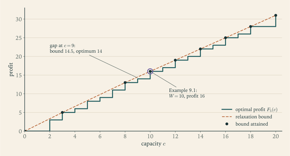
The table contains more than the answer to one question. Its last row is the optimal value for every capacity from \(0\) to \(10\) : a pack of \(9\) kilograms can carry profit \(14\) , and the tenth kilogram is worth \(2\) . The fifth item, the most valuable single item, changes nothing in its row: every entry of row 5 equals the entry above it.
9.2 What the table costs
The table has \((n+1)(W+1)\) entries. Example 1.3 measured what that means: multiplying the weights and the capacity by \(1024\) adds ten bits to each of those numbers and multiplies the table by about a thousand. In the terms of Definition 1.5 the algorithm is pseudo-polynomial. For a warehouse problem with capacities in the thousands it is excellent; for a cryptographic subset-sum instance with two-hundred-digit numbers it is useless, and no contradiction with Proposition 1.11 arises, because NP-hardness concerns exactly those instances whose numbers are large.
Two refinements are worth knowing. Row \(k\) depends only on row \(k-1\) , so if only the optimal value is wanted a single row suffices, updated in place for \(c=W,W-1,\dots,w_k\) ; the descending order guarantees that \(F(c-w_k)\) still holds the value from the previous row when it is used. And the roles of weight and profit can be exchanged, which matters when the profits are small numbers and the weights are not.
Common mistake. Updating a single row in ascending order of capacity. Then \(F(c-w_k)\) has already been updated for item \(k\) when it is read, so the item can be counted again, and the table computes the answer to a different problem, in which each item may be used any number of times. With the items of Example 9.1 and ascending updates, the entry for capacity \(6\) becomes \(10\) , from two copies of item 2, where the correct value is \(F_5(6)=9\) ; and the entry for capacity \(9\) becomes \(15\) , from three copies, in place of \(14\) . Descending order solves the 0–1 problem; ascending order solves the unbounded one of Section 9.6.
9.3 A table indexed by profit
For \(k=0,\dots,n\) and \(q=0,1,\dots,P\) , where \(P=p_1+\dots+p_n\) , let \(G_k(q)\) be the smallest total weight of a subset of the first \(k\) items whose total profit is exactly \(q\) , and \(\infty\) if there is no such subset.
Theorem 9.2 (knapsack recursion by profit). \(G_0(0)=0\) and \(G_0(q)=\infty\) for \(q\ge 1\) ; for \(k\ge 1\) ,
where the second term is present only if \(p_k\le q\) . The optimal value of the knapsack problem is the largest \(q\) with \(G_n(q)\le W\) . The table is computed in \(O(nP)\) operations, and \(P\le n\,p_{\max}\) , where \(p_{\max}\) is the largest profit.
Proof. The recursion follows from the same case distinction as in Theorem 9.1: a lightest subset of the first \(k\) items with profit exactly \(q\) either omits item \(k\) , and is a lightest such subset of the first \(k-1\) items, or contains it, and then the rest is a lightest subset of the first \(k-1\) items with profit exactly \(q-p_k\) . A profit \(q\) is attainable within the capacity exactly when some subset with profit \(q\) has weight at most \(W\) , that is, when \(G_n(q)\le W\) .
Example 9.2: Small profits, large weights
Four shipments have profits \(3,4,5,2\) and weights \(40,50,70,30\) , and the truck carries \(W=100\) . A table by weight would have \(101\) columns; a table by profit has \(P+1=15\) . Its last row is
| \(q\) | \(0\) | \(1\) | \(2\) | \(3\) | \(4\) | \(5\) | \(6\) | \(7\) | \(8\) | \(9\) | \(10\) | \(11\) | \(12\) | \(13\) | \(14\) |
|---|---|---|---|---|---|---|---|---|---|---|---|---|---|---|---|
| \(G_4(q)\) | \(0\) | \(\infty\) | \(30\) | \(40\) | \(50\) | \(70\) | \(80\) | \(90\) | \(110\) | \(120\) | \(140\) | \(150\) | \(160\) | \(\infty\) | \(190\) |
For instance \(G_4(7)=90\) : profit \(7\) arises as \(3+4\) with weight \(90\) or as \(5+2\) with weight \(100\) , and the lighter is recorded. No subset has profit \(1\) or \(13\) . The largest \(q\) with \(G_4(q)\le 100\) is \(q=7\) , so the optimal value is \(7\) , attained by shipments 1 and 2 with ten units of capacity to spare. Shipments 3 and 4 also give profit \(7\) and fill the truck exactly; the profit table prefers the lighter of two equally profitable sets, which is the natural tie-break for it.
9.4 Greedy, and a guarantee of one half
Long before a table is filled, the greedy rule of Proposition 7.5 has produced a feasible solution: the items before the critical one. How bad can it be?
Example 9.3: Greedy at its worst, and repaired
Let the capacity be \(W=100\) and let there be two items: the first with profit \(2\) and weight \(1\) , the second with profit \(100\) and weight \(100\) . The ratios are \(2\) and \(1\) , so greedy takes the first item; the second no longer fits. Greedy earns \(2\) and the optimum is \(100\) . Replacing \(100\) by a larger number makes the ratio as bad as one likes: plain greedy has no guarantee at all.
The repair is to compare the greedy set with the critical item taken alone, and keep the better. Here the critical item is the second, worth \(100\) , and the repaired rule returns the optimum.
For a second instance, let \(W=100\) with three items: profit \(52\) and weight \(51\) ; profit \(50\) and weight \(50\) ; profit \(50\) and weight \(50\) . The ratios are about \(1.02\) , \(1\) , \(1\) . Greedy takes the first item, and the second is critical. The repaired rule returns the better of \(52\) and \(50\) , namely \(52\) . The optimum is the last two items together, worth \(100\) . The ratio is \(0.52\) , barely more than one half, and by making the weights \(M+1,M,M\) and the profits \(M+2,M,M\) with capacity \(2M\) it can be brought as close to one half as desired.
Theorem 9.3 (the repaired greedy rule is a half-approximation). Suppose every item fits by itself, \(w_j\le W\) , and not all items fit together. Let the items be numbered by decreasing ratio, let \(s\) be the critical item, and let \(z_G=\max\{p_1+\dots+p_{s-1},\ p_s\}\) . Then
Proof. By Proposition 7.5 the relaxation’s optimal value is \(z_{LP}=p_1+\dots+p_{s-1}+x_sp_s\) with \(0\le x_s<1\) , so \(z_{LP}\le(p_1+\dots+p_{s-1})+p_s\le 2z_G\) . Both candidate solutions are feasible: the items before \(s\) fit by the definition of the critical item, and item \(s\) fits alone by hypothesis. Finally \(z^\star\le z_{LP}\) by Proposition 1.3.
The proof compares the heuristic with the relaxation, not with the unknown optimum. This is the standard way to prove an approximation guarantee, and it also delivers a guarantee for the instance at hand, \(z_G/z_{LP}\) , which is usually far better than one half. Example 9.3 shows that the constant in the theorem cannot be improved for this rule.
9.5 Rounding the profits: a fully polynomial approximation scheme
The profit table of Theorem 9.2 has \(nP+n\) entries, and it is large only because the profits are large numbers. Suppose the profits are divided by some \(K>0\) and rounded down. The table shrinks by a factor of about \(K\) , and each item’s profit is misrepresented by less than \(K\) . A solution that is optimal for the rounded profits can therefore be worse than the true optimum by less than \(nK\) . Choosing \(K\) so that \(nK\) is a small fraction of the optimum gives a small relative error.
The scaling algorithm with tolerance \(0<\varepsilon<1\) : discard items with \(w_j>W\) ; set \(K=\varepsilon\,p_{\max}/n\) and \(p'_j=\lfloor p_j/K\rfloor\) ; compute, by the profit recursion with profits \(p'_j\) and the original weights, a subset \(S'\) that is optimal for the rounded profits; return \(S'\) .
Theorem 9.4 (guarantee of the scaling algorithm). The set \(S'\) returned by the scaling algorithm is feasible and satisfies
The algorithm runs in \(O(n^3/\varepsilon)\) operations.
Proof. Feasibility is immediate, since the weights and the capacity were not changed. Let \(O\) be an optimal set for the original profits. Because \(p'_j\le p_j/K<p'_j+1\) ,
The second inequality holds because \(S'\) is optimal for the rounded profits and \(O\) is feasible. By the choice of \(K\) , \(nK=\varepsilon\,p_{\max}\) , and \(p_{\max}\le z^\star\) because the most profitable item fits by itself. Hence the profit of \(S'\) is at least \(z^\star-\varepsilon z^\star\) .
For the running time, each rounded profit is at most \(p_{\max}/K=n/\varepsilon\) , so the rounded total is at most \(n^2/\varepsilon\) , and by Theorem 9.2 the table takes \(O(n\cdot n^2/\varepsilon)\) operations.
Definition 9.5 (approximation schemes). For a maximization problem, a polynomial-time approximation scheme is a family of algorithms, one for each \(\varepsilon>0\) , each running in time polynomial in the input length and returning a feasible solution of value at least \((1-\varepsilon)z^\star\) . It is fully polynomial if the running time is also bounded by a polynomial in \(1/\varepsilon\) .
Theorem 9.4 says that the knapsack problem has a fully polynomial approximation scheme. The running time \(O(n^3/\varepsilon)\) no longer involves the magnitudes of the numbers at all: the dependence on \(p_{\max}\) has been traded for a dependence on the accuracy demanded.
Example 9.4: The same instance at two tolerances
Take four items with profits \(2312\) , \(2408\) , \(1532\) , \(1297\) and weights \(11\) , \(12\) , \(8\) , \(7\) , with \(W=26\) . The profit table for the exact problem would have a column for each profit up to \(7549\) . The optimum, which we know from enumeration, is items \(1,3,4\) with weight \(26\) and profit \(5141\) ; the next best set is items \(1,2\) with profit \(4720\) .
Tolerance \(\varepsilon=\tfrac12\) . Here \(K=\tfrac12\cdot 2408/4=301\) , and the rounded profits are \(\lfloor 2312/301\rfloor=7\) , \(8\) , \(5\) , \(4\) , with total \(24\) . The table has \(25\) columns. Among sets of weight at most \(26\) , the largest rounded profit is \(7+5+4=16\) , from items \(1,3,4\) ; items \(1,2\) give \(15\) . The algorithm returns items \(1,3,4\) , the true optimum. The guarantee was only \(50\) percent.
Tolerance \(\varepsilon=\tfrac9{10}\) . Now \(K=541.8\) and the rounded profits are \(4,4,2,2\) . Items \(1,2\) and items \(1,3,4\) both have rounded profit \(8\) ; the rounding can no longer tell them apart, and the profit table records the lighter, items \(1,2\) with weight \(23\) . The algorithm returns profit \(4720\) , which is \(91.8\) percent of the optimum. The guarantee was \(10\) percent, and the loss of \(421\) is well inside the allowed \(\varepsilon\,p_{\max}\approx 2167\) .
Coarser rounding gives a smaller table and a weaker answer, and the theorem bounds the loss in advance.
9.6 Variants, a second view of the table, and the limits of the idea
Unbounded knapsack. If any number of copies of each item may be taken, the item index is no longer needed in the state: with \(F(c)\) the best profit for capacity \(c\) ,
computed for \(c=1,2,\dots,W\) in ascending order. This is the computation that the Common mistake of Section 9.2 performs by accident.
Example 9.5: Cutting a ten-metre bar
A bar of length \(10\) can be cut into pieces of lengths \(3\) , \(4\) , and \(5\) , which sell for \(4\) , \(6\) , and \(7\) ; any number of each may be cut. The recursion gives
| \(c\) | \(0\) | \(1\) | \(2\) | \(3\) | \(4\) | \(5\) | \(6\) | \(7\) | \(8\) | \(9\) | \(10\) |
|---|---|---|---|---|---|---|---|---|---|---|---|
| \(F(c)\) | \(0\) | \(0\) | \(0\) | \(4\) | \(6\) | \(7\) | \(8\) | \(10\) | \(12\) | \(13\) | \(14\) |
For instance \(F(8)=\max\{F(5)+4,\ F(4)+6,\ F(3)+7\}=\max\{11,12,11\}=12\) , two pieces of length \(4\) . And \(F(10)=\max\{F(7)+4,\ F(6)+6,\ F(5)+7\}=14\) , attained three ways; one is the pieces \(3,3,4\) with value \(4+4+6\) . The piece of length \(4\) has the best value per metre, \(1.5\) , so the relaxation bound is \(15\) , and the table shows that \(14\) is the best achievable: two pieces of length \(4\) leave \(2\) metres of waste, and no combination uses the bar fully at that rate. This small problem is the pricing step of the cutting-stock method of Chapter 10.
The table is a longest path. Make a node for each state \((k,c)\) and, from each node, an arc to \((k+1,c)\) of length \(0\) and, if \(w_{k+1}\le c\) , an arc to \((k+1,c-w_{k+1})\) of length \(p_{k+1}\) . The network is acyclic, since every arc increases \(k\) , and a path from \((0,W)\) through all \(n\) levels is a sequence of decisions whose length is the profit collected. The knapsack optimum is the longest such path, and filling the table is the single pass in topological order of Section 2.4. Dynamic programming over a finite state space is always a shortest- or longest-path computation in an acyclic network; what varies from problem to problem is whether a small enough state space exists.
Limits. For the knapsack problem it does, provided the numbers are small. For two knapsack constraints at once the state must record two remaining capacities, and the table has \(nW_1W_2\) entries; with \(m\) constraints it has \(n\prod_iW_i\) , and the method fails for general integer programs. For strongly NP-hard problems such as vertex cover or the travelling salesman problem, defined in Chapter 1, a pseudo-polynomial algorithm would be a polynomial one, because all their numbers are small; so none exists unless P equals NP, and for the same reason they have no fully polynomial approximation scheme. What can be proved for them is the subject of the last chapter.
Exercises
-
Fill in the table \(F_k(c)\) for items with profits \((4,5,7,3)\) and weights \((2,3,4,1)\) and capacity \(W=6\) , state the optimal value, and recover an optimal subset by backtracking, showing each comparison.
Solution
The table, with capacities \(0\) to \(6\) across:
\(k\) \(0\) \(1\) \(2\) \(3\) \(4\) \(5\) \(6\) \(0\) \(0\) \(0\) \(0\) \(0\) \(0\) \(0\) \(0\) \(1\) \(0\) \(0\) \(4\) \(4\) \(4\) \(4\) \(4\) \(2\) \(0\) \(0\) \(4\) \(5\) \(5\) \(9\) \(9\) \(3\) \(0\) \(0\) \(4\) \(5\) \(7\) \(9\) \(11\) \(4\) \(0\) \(3\) \(4\) \(7\) \(8\) \(10\) \(12\) Sample entries: \(F_2(5)=\max\{F_1(5),F_1(2)+5\}=\max\{4,9\}=9\) ; \(F_3(6)=\max\{F_2(6),F_2(2)+7\}=\max\{9,11\}=11\) ; \(F_4(6)=\max\{F_3(6),F_3(5)+3\}=\max\{11,12\}=12\) .
The optimal value is \(F_4(6)=12\) . Backtracking from \((4,6)\) : \(F_4(6)=12\ne F_3(6)=11\) , so item 4 is in, and the capacity becomes \(5\) . \(F_3(5)=9=F_2(5)\) , so item 3 is out. \(F_2(5)=9\ne F_1(5)=4\) , so item 2 is in, and the capacity becomes \(2\) . \(F_1(2)=4\ne F_0(2)=0\) , so item 1 is in. The optimal subset is items \(1,2,4\) , with weight \(2+3+1=6\) and profit \(4+5+3=12\) . The item with the largest profit, item 3, is not used.
-
Using only the table of Example 9.1, state the optimal value and an optimal subset when the capacity is \(7\) and only the first three items are available, and when the capacity is \(9\) and all five items are available.
Answer
\(F_3(7)=11\) : since \(F_3(7)=F_2(7)\) item 3 is out, \(F_2(7)\ne F_1(7)\) puts item 2 in, and \(F_1(4)=6\) puts item 1 in; the subset is items \(1,2\) with weight \(7\) . \(F_5(9)=14\) : rows 5 and 4 agree with row 3 at capacity \(9\) , \(F_3(9)=14\ne F_2(9)=11\) puts item 3 in, and at capacity \(4\) item 1 is in; the subset is items \(1,3\) with weight \(9\) .
-
For the instance of Exercise 1 compute the last row \(G_4(q)\) of the profit table for \(q=0,\dots,19\) , and confirm the optimal value found in Exercise 1.
Solution
The profits are \((4,5,7,3)\) with total \(P=19\) and the weights \((2,3,4,1)\) . Each attainable profit is the profit of one or more subsets, and \(G_4(q)\) is the least weight among them. The single items give \(G(4)=2\) , \(G(5)=3\) , \(G(7)=4\) , \(G(3)=1\) . The pairs: items \(1,2\) give profit \(9\) with weight \(5\) ; items \(1,3\) give \(11\) with weight \(6\) ; items \(1,4\) give \(7\) with weight \(3\) , lighter than item 3 alone; items \(2,3\) give \(12\) with weight \(7\) ; items \(2,4\) give \(8\) with weight \(4\) ; items \(3,4\) give \(10\) with weight \(5\) . The triples: items \(1,2,3\) give \(16\) with weight \(9\) ; items \(1,2,4\) give \(12\) with weight \(6\) , lighter than items \(2,3\) ; items \(1,3,4\) give \(14\) with weight \(7\) ; items \(2,3,4\) give \(15\) with weight \(8\) . All four give \(19\) with weight \(10\) .
\(q\) \(0\) \(3\) \(4\) \(5\) \(7\) \(8\) \(9\) \(10\) \(11\) \(12\) \(14\) \(15\) \(16\) \(19\) \(G_4(q)\) \(0\) \(1\) \(2\) \(3\) \(3\) \(4\) \(5\) \(5\) \(6\) \(6\) \(7\) \(8\) \(9\) \(10\) and \(G_4(q)=\infty\) for \(q=1,2,6,13,17,18\) . The largest \(q\) with \(G_4(q)\le 6\) is \(q=12\) , attained with weight \(6\) by items \(1,2,4\) . This confirms the optimal value \(12\) of Exercise 9.1.
-
Prove that \(F_k(c)\) is nondecreasing in \(c\) for fixed \(k\) and nondecreasing in \(k\) for fixed \(c\) , directly from the definition of \(F_k(c)\) and not from the recursion.
Solution
By definition \(F_k(c)\) is the largest profit of a subset of the first \(k\) items with weight at most \(c\) .
Monotone in \(c\) . If \(c\le c'\) , every subset of weight at most \(c\) has weight at most \(c'\) . So the family of subsets over which \(F_k(c')\) is a maximum contains the family for \(F_k(c)\) , and a maximum over a larger family is at least as large: \(F_k(c)\le F_k(c')\) .
Monotone in \(k\) . A subset of the first \(k-1\) items is also a subset of the first \(k\) items, with the same weight. So the family for \(F_k(c)\) contains the family for \(F_{k-1}(c)\) , and \(F_{k-1}(c)\le F_k(c)\) .
Both families are nonempty, since the empty set has weight \(0\le c\) , so the maxima exist and are at least \(0\) .
Both facts are visible in the table of Example 9.1: entries do not decrease along a row or down a column. They are useful checks when filling a table by hand, and the first gives the reading of the last row as a staircase in Figure 9.1. The profit table behaves differently: \(G_k(q)\) is not monotone in \(q\) , because it concerns exact profits. In Exercise 9.3, \(G_4(6)=\infty\) while \(G_4(7)=3\) .
-
A single array \(F(0),\dots,F(W)\) is updated for each item \(k\) by the rule \(F(c)\leftarrow\max\{F(c),F(c-w_k)+p_k\}\) . Explain why processing \(c\) in descending order computes row \(k\) of the table of Theorem 9.1, and trace both orders for the single item with profit \(5\) and weight \(3\) and \(W=7\) .
Solution
Suppose that before item \(k\) is processed the array holds row \(k-1\) : \(F(c)=F_{k-1}(c)\) for all \(c\) . Process \(c=W,W-1,\dots,w_k\) . When position \(c\) is updated, position \(c-w_k<c\) has not yet been touched in this pass, so it still holds \(F_{k-1}(c-w_k)\) , and the update computes \(\max\{F_{k-1}(c),F_{k-1}(c-w_k)+p_k\}=F_k(c)\) . Positions below \(w_k\) are left alone, and for them \(F_k(c)=F_{k-1}(c)\) . So after the pass the array holds row \(k\) .
Trace, descending. Start with zeros. \(F(7)\leftarrow\max\{0,F(4)+5\}=5\) ; \(F(6)\leftarrow F(3)+5=5\) ; \(F(5)\leftarrow 5\) ; \(F(4)\leftarrow F(1)+5=5\) ; \(F(3)\leftarrow F(0)+5=5\) . The array is \((0,0,0,5,5,5,5,5)\) : the item is used at most once.
Trace, ascending. \(F(3)\leftarrow F(0)+5=5\) ; \(F(4)\leftarrow F(1)+5=5\) ; \(F(5)\leftarrow 5\) ; \(F(6)\leftarrow F(3)+5=10\) , because \(F(3)\) was already raised to \(5\) in this pass; \(F(7)\leftarrow F(4)+5=10\) . The array is \((0,0,0,5,5,5,10,10)\) : at capacity \(6\) the single item has been counted twice. Ascending order solves the problem in which the item may be repeated.
-
Solve the unbounded knapsack problem with item weights \((2,5,7)\) , profits \((3,8,12)\) , and capacity \(12\) by the recursion of Section 9.6, giving \(F(c)\) for \(c=0,\dots,12\) and an optimal multiset of items.
Solution
With weights \((2,5,7)\) and profits \((3,8,12)\) , compute \(F(c)=\max\{F(c-2)+3,\ F(c-5)+8,\ F(c-7)+12\}\) over the terms with nonnegative argument, and \(F(0)=F(1)=0\) .
\(c\) \(0\) \(1\) \(2\) \(3\) \(4\) \(5\) \(6\) \(7\) \(8\) \(9\) \(10\) \(11\) \(12\) \(F(c)\) \(0\) \(0\) \(3\) \(3\) \(6\) \(8\) \(9\) \(12\) \(12\) \(15\) \(16\) \(18\) \(20\) For example \(F(9)=\max\{F(7)+3,\ F(4)+8,\ F(2)+12\}=\max\{15,14,15\}=15\) and \(F(12)=\max\{F(10)+3,\ F(7)+8,\ F(5)+12\}=\max\{19,20,20\}=20\) . The optimal value is \(20\) , attained by one item of weight \(5\) and one of weight \(7\) , which fill the capacity exactly: \(8+12=20\) .
The item with the best ratio is the third, at \(12/7\approx 1.71\) , so the relaxation bound is \(12\cdot 12/7\approx 20.57\) , and the bound rounds down to the optimum. Using the best-ratio item greedily would take one copy and then two copies of the first item, with weight \(11\) and profit \(18\) .
-
The subset-sum problem asks whether some subset of positive integers \(a_1,\dots,a_n\) has total exactly \(T\) . Show how to decide it with the table of Theorem 9.1, state the running time, and apply your method to the numbers \(3,5,6,9\) with \(T=14\) and with \(T=16\) .
Hint
Use each number as both weight and profit, with capacity \(T\) : the answer is yes exactly when \(F_n(T)=T\) . The running time is \(O(nT)\) , pseudo-polynomial. For \(3,5,6,9\) : \(T=14\) is attainable, as \(5+9\) or \(3+5+6\) ; \(T=16\) is not, since the subset sums are \(3,5,6,8,9,11,12,14,15,17,18,20,23\) .
-
For the items of Example 9.1 with capacity \(10\) , order the items by ratio, find the critical item, compute \(z_{LP}\) and the value \(z_G\) of Theorem 9.3, and compare the guarantee \(z_G/z_{LP}\) with the true ratio \(z_G/z^\star\) .
Solution
The ratios are \(6/4=1.5\) , \(5/3\approx 1.67\) , \(8/5=1.6\) , \(3/2=1.5\) , \(9/6=1.5\) . In decreasing order the items are \(2\) , \(3\) , and then items \(1,4,5\) tied at \(1.5\) ; keep those in index order.
Greedy takes item 2, using \(3\) of the \(10\) kilograms, then item 3, using \(5\) more, for a total of \(8\) and profit \(13\) . The next item, item 1, weighs \(4>2\) , so it is the critical item, with \(x_1=2/4\) . Hence
\[ z_{LP}=5+8+\tfrac12\cdot 6=16,\qquad z_G=\max\{13,\ 6\}=13 . \]From Example 9.1, \(z^\star=16\) . The guarantee available without knowing the optimum is \(z_G/z_{LP}=13/16\approx 0.81\) , and here it equals the true ratio \(z_G/z^\star\) , because the relaxation bound happens to be exact at capacity \(10\) , one of the points where the two curves of Figure 9.1 touch.
Greedy stopped two kilograms short. Continuing past the critical item to any later item that still fits, here item 4, would give items \(2,3,4\) with profit \(16\) , the optimum. That extension is harmless and usually helpful, but Theorem 9.3 does not need it and its worst-case ratio is still one half.
-
Construct, for a given integer \(M\ge 2\) , a knapsack instance with three items on which the repaired greedy rule of Theorem 9.3 returns \(M+2\) while the optimum is \(2M\) , and verify the hypotheses of the theorem for your instance.
Hint
Capacity \(2M\) ; item 1 with weight \(M+1\) and profit \(M+2\) ; items 2 and 3 with weight \(M\) and profit \(M\) . Each item fits alone, not all fit together, the ratios are \((M+2)/(M+1)>1=1\) , the critical item is the second, and \(z_G=\max\{M+2,M\}\) while items 2 and 3 together give \(2M\) .
-
Run the scaling algorithm with \(\varepsilon=\tfrac12\) on the instance with profits \((60,100,120)\) , weights \((10,20,30)\) , and capacity \(50\) : give \(K\) , the rounded profits, the set returned, its true profit, and the guarantee of Theorem 9.4.
Solution
There are \(n=3\) items and \(p_{\max}=120\) , so \(K=\varepsilon\,p_{\max}/n=\tfrac12\cdot 120/3=20\) . The rounded profits are \(\lfloor 60/20\rfloor=3\) , \(\lfloor 100/20\rfloor=5\) , \(\lfloor 120/20\rfloor=6\) .
The feasible sets, with capacity \(50\) : any single item; items \(1,2\) with weight \(30\) and rounded profit \(8\) ; items \(1,3\) with weight \(40\) and rounded profit \(9\) ; items \(2,3\) with weight \(50\) and rounded profit \(11\) . All three together weigh \(60\) , too much. The largest rounded profit is \(11\) , so the algorithm returns items \(2,3\) .
Their true profit is \(100+120=220\) . The guarantee of Theorem 9.4 is that the returned set is worth at least \((1-\tfrac12)z^\star\) . In fact \(220\) is the optimum, as the list of feasible sets shows: the others are worth at most \(180\) . Because every profit here is a multiple of \(K=20\) , no rounding error occurred at all and the scaled problem was equivalent to the original, an instance of the observation in Exercise 9.18.
-
In the proof of Theorem 9.4, identify the step that would fail if the profits were rounded up instead of down, and determine whether the algorithm with rounding up still has a guarantee by examining the chain of inequalities.
Solution
With rounding up, \(p'_j=\lceil p_j/K\rceil\) , we have \(p_j\le Kp'_j<p_j+K\) . The first step of the chain in the proof, \(\sum_{j\in S'}p_j\ge K\sum_{j\in S'}p'_j\) , used \(Kp'_j\le p_j\) and now fails: the rounded profits overstate the true ones.
The conclusion survives with the errors moved to the other end of the chain. Using \(p_j>Kp'_j-K\) on \(S'\) and \(Kp'_j\ge p_j\) on an optimal set \(O\) ,
\[ \sum_{j\in S'}p_j\ >\ K\sum_{j\in S'}p'_j-nK\ \ge\ K\sum_{j\in O}p'_j-nK\ \ge\ \sum_{j\in O}p_j-nK=z^\star-nK , \]where the middle inequality is again the optimality of \(S'\) for the rounded profits. With \(K=\varepsilon\,p_{\max}/n\) this gives the same guarantee \((1-\varepsilon)z^\star\) . The table is slightly larger, since rounded profits can be as large as \(\lceil n/\varepsilon\rceil\) .
So either direction of rounding works, provided it is applied consistently and the error per item is less than \(K\) . What matters is that the optimal set and the returned set are both measured, in the rounded problem, to within \(K\) per item.
-
Explain what is wrong with this proposal: “To handle large weights, divide every weight and the capacity by \(K\) , round down, and run the weight table of Theorem 9.1 on the rounded data.” Give a two-item instance on which the proposal returns an infeasible set.
Solution
Rounding weights down understates them, so a set that fits in the rounded problem may not fit in the real one. Feasibility, unlike the objective, cannot be traded for speed: an answer that is \(5\) percent overweight is not a slightly worse answer, it is not an answer.
For an instance, take two items of weight \(6\) and profit \(1\) each, capacity \(11\) , and \(K=4\) . The rounded weights are \(\lfloor 6/4\rfloor=1\) and the rounded capacity is \(\lfloor 11/4\rfloor=2\) . In the rounded problem both items fit, with rounded weight \(2\le 2\) , so the proposal returns both items. Their true weight is \(12>11\) : infeasible.
Rounding the weights up and the capacity down preserves feasibility but can lose every good solution: with the same items and \(K=4\) , the rounded weights are \(2\) and the rounded capacity \(2\) , so only one item is allowed, which here happens to be correct; with capacity \(12\) the rounded capacity is \(3\) , still one item, although both fit. No guarantee on profit survives. The asymmetry is the reason approximation schemes for knapsack round profits and leave the weights exact.
-
Explain why the existence of a fully polynomial approximation scheme for the knapsack problem does not imply that P equals NP, by examining the running time needed to guarantee an exactly optimal solution when profits are integers.
Hint
With integer profits, a solution of value at least \((1-\varepsilon)z^\star\) is optimal as soon as \(\varepsilon z^\star<1\) . That needs \(\varepsilon<1/z^\star\) , and the running time \(O(n^3/\varepsilon)\) becomes \(O(n^3z^\star)\) , which is pseudo-polynomial: polynomial in the magnitude of the profits, not in their length. The scheme is polynomial for each fixed tolerance, not for the tolerance that exactness requires.
-
Draw the acyclic network of Section 9.6 for the instance with profits \((3,4)\) , weights \((1,2)\) , and \(W=2\) , list all paths from \((0,2)\) through both levels with their lengths, and identify the longest.
Answer
Nodes \((0,2)\) ; \((1,2)\) and \((1,1)\) ; \((2,2)\) , \((2,0)\) , \((2,1)\) . Arcs: from \((0,2)\) to \((1,2)\) with length \(0\) and to \((1,1)\) with length \(3\) ; from \((1,2)\) to \((2,2)\) with length \(0\) and to \((2,0)\) with length \(4\) ; from \((1,1)\) to \((2,1)\) with length \(0\) , item 2 being too heavy there. The three paths have lengths \(0\) , \(4\) , and \(3\) ; the longest, through \((1,2)\) and \((2,0)\) , takes item 2 alone for profit \(4\) .
-
For the knapsack of Example 7.2, the Dantzig bound at the root was \(52.625\) and branch-and-bound evaluated \(13\) nodes. State the number of table entries the weight recursion would compute for that instance, and discuss which method you would prefer if the capacity were \(26000\) and the weights a thousand times larger.
Hint
Four rows of \(27\) entries, \(108\) in all as in Example 1.3, or \(135\) counting the row of zeros. With capacity \(26000\) the table has more than a hundred thousand entries while the branch-and-bound tree and the cover cuts are unchanged, since they depend on the ratios and on which sets fit, not on the unit of weight.
-
The separation problem of Proposition 8.7 asks to minimize \(\sum_j(1-\bar x_j)z_j\) subject to \(\sum_jw_jz_j\ge W+1\) . Define a table \(H_k(c)\) , the least cost of a subset of the first \(k\) items with weight at least \(c\) , write its recursion, and say what its running time is.
Hint
\(H_0(0)=0\) , \(H_0(c)=\infty\) for \(c\ge 1\) , and \(H_k(c)=\min\{H_{k-1}(c),\ H_{k-1}(\max\{c-w_k,0\})+(1-\bar x_k)\}\) for \(c=0,\dots,W+1\) . A violated cover exists exactly when \(H_n(W+1)<1\) . The table has \((n+1)(W+2)\) entries.
-
A knapsack problem has two constraints, weight at most \(W\) and volume at most \(V\) . Write the recursion for \(F_k(c,d)\) , give the number of table entries, and compute the optimal value for items with (profit, weight, volume) equal to \((5,1,2)\) , \((4,2,1)\) , \((6,2,2)\) and \(W=3\) , \(V=3\) .
Solution
Let \(F_k(c,d)\) be the best profit from the first \(k\) items with weight at most \(c\) and volume at most \(d\) . Then \(F_0(c,d)=0\) and, writing \(w_k\) and \(v_k\) for the weight and volume of item \(k\) ,
\[ F_k(c,d)=\max\{F_{k-1}(c,d),\ F_{k-1}(c-w_k,\,d-v_k)+p_k\}, \]with the second term present only when \(w_k\le c\) and \(v_k\le d\) . The proof is that of Theorem 9.1 with a two-component capacity. The table has \((n+1)(W+1)(V+1)\) entries, here \(4\cdot 4\cdot 4=64\) .
For the instance, it is quicker to list subsets. Items 1 and 2 together have weight \(3\) and volume \(3\) : feasible, profit \(9\) . Items 1 and 3 have weight \(3\) and volume \(4\) : too bulky. Items 2 and 3 have weight \(4\) : too heavy. All three are too heavy. The single items are worth \(5\) , \(4\) , \(6\) . So \(F_3(3,3)=9\) , from items 1 and 2. The recursion agrees: \(F_3(3,3)=\max\{F_2(3,3),\ F_2(1,1)+6\}=\max\{9,\ 0+6\}=9\) , since with weight \(1\) and volume \(1\) neither of the first two items fits.
The most profitable item is excluded because it is second-worst in both resources. With one constraint a ratio orders the items; with two there is no single ratio, which is one reason the greedy bound of Proposition 7.5 has no simple analogue here.
-
Prove that if all profits are multiples of an integer \(g\ge 1\) then the profit table of Theorem 9.2 needs only the columns that are multiples of \(g\) , and explain how this observation is the scaling algorithm without the rounding error.
Hint
By induction on \(k\) , every profit attainable from the first \(k\) items is a sum of multiples of \(g\) , so \(G_k(q)=\infty\) unless \(g\) divides \(q\) , and the recursion only ever reads columns \(q\) and \(q-p_k\) , both multiples of \(g\) or both not. Keeping only the multiples of \(g\) is the same as dividing every profit by \(g\) , exactly. The scaling algorithm divides by \(K\) and rounds down, which makes the profits multiples of \(K\) at the price of an error below \(K\) per item; when the profits are already multiples of \(K\) there is no error, as in Exercise 9.10.