A telecommunications planner must place monitoring equipment on network nodes so that every link has a monitor at one end, using as few monitors as possible. This is the vertex cover problem, NP-hard by Theorem 1.10, and the network has forty thousand links. Branch-and-cut may or may not finish. The planner’s real question is different from “what is the optimum”: it is “can I have, by this afternoon, a placement that is provably not much worse than the optimum, and how much worse might it be?”
That question has precise answers. For vertex cover, two different algorithms, each a few lines long, return a cover at most twice the minimum size, with proof. For covering problems with arbitrary sets the best possible guarantee grows like a logarithm. For the travelling salesman problem the answer depends on a hypothesis: with the triangle inequality a factor of two is easy, and without it no factor at all is achievable unless P equals NP. In every case the proof has the same skeleton as the proofs of this book so far: a feasible solution on one side, a bound from a relaxation on the other.
The second half of the chapter returns to bounds. Lagrangian relaxation and column generation produce bounds stronger than a compact linear programming relaxation by letting a combinatorial subproblem, a knapsack or a shortest path, do part of the work. The chapter closes by setting side by side the methods of the whole book and the evidence each one hands over with its answer.
10.1 What a guarantee is
Definition 10.1 (approximation algorithm). For a minimization problem and a number \(\rho\ge 1\) , a polynomial algorithm is a \(\rho\) -approximation algorithm if on every instance it returns a feasible solution of cost at most \(\rho\) times the optimal cost. For a maximization problem and a number \(0<\alpha\le 1\) , it is an \(\alpha\) -approximation algorithm if it returns a feasible solution of value at least \(\alpha\) times the optimal value. The number \(\rho\) or \(\alpha\) is the approximation ratio, or performance guarantee.
The repaired greedy rule of Theorem 9.3 is a \(\tfrac12\) -approximation algorithm for knapsack, and the scaling algorithm of Theorem 9.4 is a \((1-\varepsilon)\) -approximation algorithm for each \(\varepsilon\) . A guarantee is a statement about every instance, proved without knowing the optimum. Since the optimum is unknown, every such proof compares the algorithm’s output with a bound that can be computed: the value of a relaxation, or of a dual solution, or of some combinatorial object such as a matching. Finding the right bound is the whole art.
10.2 Vertex cover, twice
Let \(G=(V,E)\) be a graph. A matching is maximal if no edge can be added to it; a maximal matching is found by scanning the edges once and keeping each edge whose endpoints are both still unmatched. It need not be a maximum matching.
Theorem 10.2 (vertex cover from a maximal matching). Let \(M\) be a maximal matching and let \(C\) be the set of all \(2\lvert M\rvert\) endpoints of its edges. Then \(C\) is a vertex cover, and \(\lvert C\rvert\) is at most twice the minimum size of a vertex cover.
Proof. If some edge had neither endpoint in \(C\) , both its endpoints would be unmatched and it could be added to \(M\) , contradicting maximality; so \(C\) is a cover. By Lemma 4.2 every vertex cover has at least \(\lvert M\rvert\) nodes, so the minimum size is at least \(\lvert M\rvert=\tfrac12\lvert C\rvert\) .
The bound used is the matching bound of Chapter 4, which in bipartite graphs is exact, by König’s theorem, and in general graphs is off by a factor of at most two, which is what the theorem exploits. The second algorithm uses a linear program and handles weights. Let each node have a weight \(w_v\ge 0\) ; the weighted vertex cover problem asks for a cover of least total weight, and its relaxation is
Theorem 10.3 (vertex cover by rounding). Let \(x^\star\) be an optimal solution of the relaxation and let \(C=\{v:x^\star_v\ge\tfrac12\}\) . Then \(C\) is a vertex cover of weight at most \(2z_{LP}\) , hence at most twice the minimum weight of a vertex cover.
Proof. For each edge \(vv'\) , \(x^\star_v+x^\star_{v'}\ge 1\) , so at least one of the two values is at least \(\tfrac12\) and that endpoint is in \(C\) . For the weight, each \(v\in C\) has \(1\le 2x^\star_v\) , so \(\sum_{v\in C}w_v\le\sum_{v\in C}2w_vx^\star_v\le 2z_{LP}\) . Finally \(z_{LP}\) is at most the minimum weight of a cover, by the minimization form of Proposition 1.3.
Example 10.1: Two algorithms on two graphs
A tree. Let the graph have edges \(12\) , \(23\) , \(34\) , \(45\) , \(26\) , \(47\) . Nodes \(2\) and \(4\) touch every edge, and no single node does, so the minimum cover has size \(2\) .
Scanning the edges in the order given, the matching algorithm keeps \(12\) , rejects \(23\) because node \(2\) is matched, keeps \(34\) , and rejects \(45\) , \(26\) , and \(47\) . The maximal matching is \(\{12,34\}\) and the cover is \(\{1,2,3,4\}\) , of size \(4\) : exactly twice the optimum, so the factor in Theorem 10.2 cannot be improved for this algorithm. The matching still certifies something useful: no cover has fewer than \(2\) nodes.
The graph is bipartite, so by Corollary 6.10 and Theorem 6.7 the relaxation has integral vertices. The simplex method returns \(x^\star_2=x^\star_4=1\) and zero elsewhere, with \(z_{LP}=2\) , and rounding returns \(\{2,4\}\) , the optimum.
The two triangles. Now take the graph of Example 1.5, with all weights \(1\) . Its minimum cover has \(4\) nodes. The relaxation’s optimal solution has every \(x^\star_v=\tfrac12\) and \(z_{LP}=3\) . Rounding puts every node in the cover: \(6\) nodes, exactly \(2z_{LP}\) , and \(1.5\) times the optimum. The scan for a maximal matching keeps \(12\) , \(35\) , and \(46\) , and its cover is again all six nodes.
Change the weights to \(w=(3,1,1,1,1,3)\) , making nodes \(1\) and \(6\) expensive. The relaxation’s solution becomes \(x^\star=(0,1,1,1,1,0)\) with \(z_{LP}=4\) , an integer vector, and rounding returns the cover \(\{2,3,4,5\}\) of weight \(4\) , which is optimal because it meets the bound. The matching algorithm cannot see weights at all.
Every run produced a bound along with its cover: a matching, or \(z_{LP}\) . The a-priori guarantee was a factor of \(2\) . The instance-specific guarantees, cover weight divided by bound, were \(2\) and \(1\) for the two algorithms on the tree, \(2\) for both on the unweighted triangles, and \(1\) for rounding on the weighted ones.
No polynomial algorithm with a guarantee better than \(2\) by a constant is known for vertex cover, and the integrality gap of this relaxation tends to \(2\) , as Exercise 5.16 showed on complete graphs, so no analysis that compares with \(z_{LP}\) can do better.
10.3 Set cover and the harmonic bound
In the set cover problem a ground set \(U\) of \(n\) elements and a family of subsets \(S_1,\dots,S_m\) with costs \(c_1,\dots,c_m>0\) are given, and the union of the family is \(U\) . A cover is a subfamily whose union is \(U\) , and the task is to find one of least total cost. Vertex cover is the special case in which the elements are the edges and the sets are the stars of the nodes; there each element lies in exactly two sets. In general there is no such limit, and the guarantee degrades.
The greedy algorithm: while some element is uncovered, choose a set minimizing its cost divided by the number of still-uncovered elements it contains; add it to the cover. Write \(H_n=1+\tfrac12+\dots+\tfrac1n\) for the \(n\) -th harmonic number, which lies between \(\ln n\) and \(1+\ln n\) .
Theorem 10.4 (greedy set cover). The greedy algorithm returns a cover of cost at most \(H_n\) times the minimum cost.
Proof. When the algorithm chooses a set \(S\) that covers \(t\) new elements, charge each of those elements the price \(c(S)/t\) . The cost of the greedy cover is the sum of all prices. Number the elements \(e_1,\dots,e_n\) in the order in which they are covered, breaking ties arbitrarily.
Fix \(k\) and consider the moment just before \(e_k\) is covered. The set \(U'\) of uncovered elements contains \(e_k,\dots,e_n\) , so \(\lvert U'\rvert\ge n-k+1\) . Let \(\mathrm{OPT}\) be the minimum cost and consider an optimal cover. Its sets cover \(U'\) , so the numbers of elements of \(U'\) they contain add up to at least \(\lvert U'\rvert\) , while their costs add up to \(\mathrm{OPT}\) . Hence at least one of them has cost per uncovered element at most \(\mathrm{OPT}/\lvert U'\rvert\) ; otherwise the total cost would exceed \(\mathrm{OPT}\) . The greedy choice is at least as good, so the price of \(e_k\) is at most \(\mathrm{OPT}/\lvert U'\rvert\le\mathrm{OPT}/(n-k+1)\) . Adding over \(k=1,\dots,n\) gives total cost at most \(\mathrm{OPT}\cdot H_n\) .
Example 10.2: Greedy takes three sets where two suffice
Let \(U=\{1,\dots,14\}\) and let every set cost \(1\) . The sets are the two rows \(R_1=\{1,\dots,7\}\) and \(R_2=\{8,\dots,14\}\) , and three blocks that straddle them: \(B_1=\{1,2,3,4,8,9,10,11\}\) , \(B_2=\{5,6,12,13\}\) , and \(B_3=\{7,14\}\) .
The two rows form a cover of cost \(2\) , which is optimal since no single set is all of \(U\) . Greedy first compares sizes \(7,7,8,4,2\) and takes \(B_1\) ; each of its eight elements is charged \(\tfrac18\) . Now each row has three uncovered elements, \(B_2\) has four, and \(B_3\) two; greedy takes \(B_2\) , charging \(\tfrac14\) to each of four elements. The uncovered elements are \(7\) and \(14\) ; each row has one of them and \(B_3\) has both; greedy takes \(B_3\) , charging \(\tfrac12\) each. The greedy cover \(\{B_1,B_2,B_3\}\) costs \(3\) , against the optimum \(2\) .
The prices add up to \(8\cdot\tfrac18+4\cdot\tfrac14+2\cdot\tfrac12=3\) , and the theorem’s bound is \(2H_{14}\approx 6.5\) . Continuing the pattern with rows of \(2^k-1\) elements and blocks of sizes \(2^k,2^{k-1},\dots,2\) makes greedy take \(k\) sets against an optimum of \(2\) , so the logarithmic growth is real and not an artefact of the proof. It is known that, unless P equals NP, no polynomial algorithm guarantees a ratio better than a constant times \(\ln n\) for set cover; greedy is essentially the best possible.
10.4 Tours: a factor of two, or none at all
Consider the travelling salesman problem on \(n\)
cities with symmetric distances \(d(i,j)\ge 0\)
. The distances are metric if they satisfy the triangle inequality \(d(i,k)\le d(i,j)+d(j,k)\)
for all cities. A spanning tree is a connected set of edges with no cycle that reaches every city; it has \(n-1\)
edges, by the equivalent descriptions of a tree proved in Discrete Mathematics (math.discrete-mathematics.tree-equivalences). A minimum spanning tree is found by the greedy rule of Kruskal: scan the edges in order of increasing length and keep each edge that joins two different components. That this rule is optimal is a standard result of graph algorithms, which we use without proof.
The tree-doubling algorithm: find a minimum spanning tree \(T\) ; walk around it, traversing each edge twice, once in each direction, so as to return to the start having visited every city; then list the cities in the order of their first appearance on the walk, and close the list into a tour.
Theorem 10.5 (tree doubling for metric distances). If the distances are metric, the tour produced by the tree-doubling algorithm has length at most twice the length of an optimal tour.
Proof. Deleting one edge from an optimal tour leaves a path through all cities, which is a spanning tree; so the minimum spanning tree has length \(d(T)\) at most the optimal tour length \(\mathrm{OPT}\) . The walk around \(T\) has length \(2d(T)\) . The tour follows the walk but skips cities already visited; each skip replaces a stretch of the walk from city \(i\) to city \(k\) by the direct edge \(ik\) , which by the triangle inequality, applied repeatedly along the stretch, is no longer. So the tour has length at most \(2d(T)\le 2\,\mathrm{OPT}\) .
An algorithm of Christofides and Serdyukov improves the factor to \(\tfrac32\) by replacing the doubling of every tree edge with a minimum-weight perfect matching on the cities of odd degree in the tree; it relies on matching in graphs that are not bipartite, which lies beyond this book. Without the triangle inequality the situation changes completely.
Proposition 10.6 (general distances admit no guarantee). If, for some constant \(\rho\ge 1\) , there is a polynomial \(\rho\) -approximation algorithm for the travelling salesman problem with arbitrary nonnegative symmetric distances, then P equals NP.
Proof. Let \(G\) be a graph on \(n\) nodes. Give each edge of \(G\) the distance \(1\) and each pair of nodes not joined in \(G\) the distance \(\rho n+1\) . If \(G\) has a Hamiltonian cycle, the optimal tour has length \(n\) and the algorithm returns a tour of length at most \(\rho n\) , which cannot use any pair of distance \(\rho n+1\) ; so the returned tour is a Hamiltonian cycle of \(G\) . If \(G\) has no Hamiltonian cycle, every tour uses such a pair and has length greater than \(\rho n\) . So comparing the length of the returned tour with \(\rho n\) decides whether \(G\) has a Hamiltonian cycle, in polynomial time, and that problem is NP-complete by Theorem 1.10.
The distances constructed in the proof violate the triangle inequality badly, which is why Theorem 10.5 is not contradicted. The pair of results shows that approximability is a property of the precise problem, hypotheses included, and not of its name.
Example 10.3: Six depots on a grid
Six depots lie at \(A=(0,0)\) , \(B=(0,3)\) , \(C=(2,5)\) , \(D=(5,4)\) , \(E=(6,1)\) , \(F=(3,1)\) , and travel is along grid lines, so distances are sums of coordinate differences and are metric.
The tree. The two shortest distances are \(d(A,B)=3\) and \(d(E,F)=3\) ; both edges are kept. Four pairs are at distance \(4\) : \(AF\) , \(BC\) , \(CD\) , and \(DE\) . Taking them in that order, \(AF\) joins the component of \(A\) and \(B\) to that of \(E\) and \(F\) ; \(BC\) adds \(C\) ; \(CD\) adds \(D\) ; and \(DE\) would close a cycle and is rejected. The tree is \(\{AB,EF,AF,BC,CD\}\) with length \(3+3+4+4+4=18\) .
The walk and the tour. Starting at \(A\) and exploring the branch through \(B\) first, the walk is \(A,B,C,D,C,B,A,F,E,F,A\) , of length \(36\) . The first appearances are \(A,B,C,D,F,E\) , and the tour \(A,B,C,D,F,E,A\) has length \(3+4+4+5+3+7=26\) .
Comparison. The best tour, found by listing all \(60\) distinct tours, is \(A,B,C,D,E,F,A\) with length \(3+4+4+4+3+4=22\) . The chain of inequalities in the proof reads \(18\le 22\le 26\le 36\) . Without knowing the optimum, the planner can assert from the tree alone that the tour of length \(26\) is within a factor \(26/18\approx 1.44\) of optimal; the truth is \(26/22\approx 1.18\) .
10.5 Lagrangian relaxation: pricing a constraint
Many hard problems are easy problems with one or two extra constraints: a knapsack with a second resource, a shortest path with a time limit, an assignment with a budget. Dropping the extra constraints gives a relaxation that is easy and weak. Lagrangian relaxation drops them and charges a price for violating them.
Write the problem as
where \(X\) is a finite set over which linear functions can be maximized efficiently and \(Dx\le d\) are the complicating constraints. For a vector of prices \(\lambda\ge 0\) , the Lagrangian subproblem and Lagrangian dual are
Proposition 10.7 (the Lagrangian bound). For every \(\lambda\ge 0\) , \(L(\lambda)\ge z^\star\) ; hence \(w_{LD}\ge z^\star\) . The function \(L\) is convex and piecewise linear. If for some \(\lambda\ge 0\) a maximizer \(\bar x\) of the subproblem satisfies \(D\bar x\le d\) and \(\lambda^{\top}(d-D\bar x)=0\) , then \(\bar x\) is optimal for the original problem.
Proof. Let \(x^\star\) be optimal for the original problem. It lies in \(X\) and \(d-Dx^\star\ge 0\) , so \(z^\star=c^{\top}x^\star\le c^{\top}x^\star+\lambda^{\top}(d-Dx^\star)\le L(\lambda)\) . For each fixed \(x\in X\) the expression \(c^{\top}x+\lambda^{\top}(d-Dx)\) is an affine function of \(\lambda\) , and \(L\) is the maximum of finitely many of them, hence convex and piecewise linear. For the last statement, \(\bar x\) is feasible, so \(c^{\top}\bar x\le z^\star\le L(\lambda)=c^{\top}\bar x+0\) .
This is the Lagrangian duality of Continuous Optimization, applied to a problem whose feasible set \(X\)
is discrete (math.continuous-optimization.lagrange-duality); the bound is weak duality, and in general there is a gap. How good is the best such bound?
Theorem 10.8 (strength of the Lagrangian dual). With the notation above,
Consequently \(z^\star\le w_{LD}\le z_{LP}\) for any formulation of \(X\) used to define \(z_{LP}\) , and \(w_{LD}=z_{LP}\) when that formulation of \(X\) is ideal.
We omit the proof, which applies linear programming duality to the right-hand side. The theorem says exactly what Lagrangian relaxation buys: the constraints kept in \(X\) are replaced by their convex hull. If the subproblem is one whose relaxation is already integral, a shortest path or an assignment, the Lagrangian bound equals the linear programming bound, and its advantage is only computational, since it is obtained by solving combinatorial subproblems. If the subproblem is a knapsack, whose relaxation is not integral, the Lagrangian bound can be strictly better.
Example 10.4: A second resource, priced
A probe can carry instruments worth \(8\) , \(7\) , \(10\) , and \(6\) , with masses \(7\) , \(3\) , \(2\) , \(3\) against a mass limit of \(11\) , and power demands \(1\) , \(2\) , \(1\) , \(4\) against a power limit of \(5\) . Enumeration shows that the best feasible payload is instruments \(1\) and \(3\) : mass \(9\) , power \(2\) , value \(z^\star=18\) . The relaxation with both constraints has value \(z_{LP}=617/25=24.68\) .
Keep the mass constraint in \(X\) and price the power constraint at \(\lambda\ge 0\) per unit. The subproblem is a knapsack with values \(c_j-\lambda D_j\) :
At \(\lambda=0\) the knapsack takes instruments \(2,3,4\) , worth \(23\) ; they need \(7\) units of power, so the solution is infeasible and \(L(0)=23\) is only a bound. At \(\lambda=1\) the adjusted values are \(7,5,9,2\) ; the best mass-feasible sets are \(\{1,3\}\) and \(\{2,3,4\}\) , both worth \(16\) , so \(L(1)=5+16=21\) . At \(\lambda=2\) the adjusted values are \(6,3,8,-2\) , the knapsack takes \(\{1,3\}\) , worth \(14\) , and \(L(2)=10+14=24\) .
Each mass-feasible set contributes one line: \(\{2,3,4\}\) gives \(23-2\lambda\) , since it overuses power by \(2\) , and \(\{1,3\}\) gives \(18+3\lambda\) , since it leaves \(3\) units unused. For \(0\le\lambda\le 1\) the first line is the largest of all twelve, and for \(1\le\lambda\le 8\) the second is. They cross at \(\lambda=1\) , so
The three bounds are \(z^\star=18\le w_{LD}=21\le z_{LP}=24.68\) . Pricing one constraint and keeping the knapsack exact removed more than half of the gap.
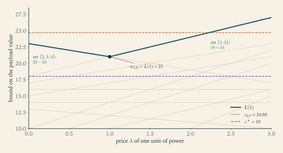
At the minimizing price the subproblem has two optimal solutions, one infeasible and one feasible but with slack, and neither satisfies the optimality test of Proposition 10.7; that is what a gap looks like. In practice \(\lambda\) is found by a subgradient method from Continuous Optimization: raise the price of a constraint the subproblem’s solution violates, lower it when there is slack, with diminishing step sizes. The feasible solutions met along the way, here \(\{1,3\}\) , serve as incumbents, and the pair \((18,21)\) is the kind of bracket a branch-and-bound method then closes.
10.6 Column generation: when the variables are too many
Chapter 8 dealt with formulations that have too many constraints. Some of the strongest formulations have too many variables instead, and the remedy is the mirror image of separation.
In the cutting-stock problem, bars of length \(\Lambda\) are cut into pieces; \(d_i\) pieces of length \(\ell_i\) are required for \(i=1,\dots,m\) , and the number of bars used is to be minimized. A pattern is a vector \(a=(a_1,\dots,a_m)\) of nonnegative integers with \(\sum_i\ell_ia_i\le\Lambda\) , describing how one bar is cut. With a variable \(y_a\) for the number of bars cut according to pattern \(a\) , the problem is
The number of patterns is astronomical for realistic data. Column generation solves the relaxation while holding only a few patterns: solve the relaxation restricted to the patterns in hand, obtaining optimal dual prices \(\pi_i\ge 0\) for the demand constraints; then look for a pattern whose dual constraint is violated.
Proposition 10.9 (pricing patterns). Let \(\pi\) be optimal dual prices for the relaxation restricted to a subset of the patterns. If
then the restricted solution is optimal for the relaxation over all patterns. Otherwise a maximizing pattern, added to the subset, may improve the relaxation.
Proof. The dual of the full relaxation maximizes \(\sum_id_i\pi_i\) subject to \(\sum_i\pi_ia_i\le 1\) for every pattern \(a\) and \(\pi\ge 0\) . If the maximum above is at most \(1\) , the prices \(\pi\) are feasible for the full dual. Their value equals the value of the restricted primal solution, by strong duality for the restricted program, and that solution is feasible for the full primal. Equal primal and dual values prove both optimal. If the maximum exceeds \(1\) , the maximizing pattern violates its dual constraint; equivalently its column has negative reduced cost \(1-\sum_i\pi_ia_i\) .
The pricing problem is an unbounded knapsack problem, solved by the recursion of Section 9.6. A hard problem has been decomposed into a linear program of modest size and a sequence of knapsacks.
Example 10.5: Cutting bars of length ten
Bars of length \(10\) are cut into pieces of lengths \(3\) , \(4\) , and \(5\) , of which \(7\) , \(5\) , and \(4\) are required. The total length required is \(21+20+20=61\) , so at least \(7\) bars are needed.
Start. Take the three patterns that cut one length only: \((3,0,0)\) , \((0,2,0)\) , \((0,0,2)\) . The restricted relaxation uses \(\tfrac73\) , \(\tfrac52\) , and \(2\) bars of them, \(\tfrac{41}6\approx 6.83\) in all, and the dual prices are \(\pi=(\tfrac13,\tfrac12,\tfrac12)\) : a piece is worth the reciprocal of the number cut from one bar.
Pricing. Maximize \(\tfrac13a_1+\tfrac12a_2+\tfrac12a_3\) subject to \(3a_1+4a_2+5a_3\le 10\) . The pattern \((2,1,0)\) , which uses the bar fully, is worth \(\tfrac23+\tfrac12=\tfrac76>1\) . Add it.
Second relaxation. With four patterns the optimal solution uses \(\tfrac34\) of a bar in pattern \((0,2,0)\) , \(2\) bars in \((0,0,2)\) , and \(\tfrac72\) bars in \((2,1,0)\) , none in \((3,0,0)\) : a total of \(\tfrac{25}4=6.25\) . The prices are \(\pi=(\tfrac14,\tfrac12,\tfrac12)\) .
Pricing again. The candidates are worth: \((3,0,0)\) , \(\tfrac34\) ; \((2,1,0)\) , \(1\) ; \((0,2,0)\) , \(1\) ; \((0,0,2)\) , \(1\) ; \((1,0,1)\) , \(\tfrac34\) ; \((0,1,1)\) , \(1\) . The maximum is \(1\) , so no pattern prices out, and by Proposition 10.9 the relaxation over all patterns has value \(6.25\) . As a check, the prices give the dual value \(7\cdot\tfrac14+5\cdot\tfrac12+4\cdot\tfrac12=6.25\) .
An integer solution. The number of bars is an integer, so at least \(\lceil 6.25\rceil=7\) bars are needed. Rounding the fractional solution up gives \(1\) bar of \((0,2,0)\) , \(2\) of \((0,0,2)\) , and \(4\) of \((2,1,0)\) : seven bars, yielding \(8\) pieces of length \(3\) , \(6\) of length \(4\) , and \(4\) of length \(5\) , which meets every demand. Seven bars is optimal.
Only four of the patterns were ever written down. Rounding up worked here because the fractional solution had few fractional entries; in general a relaxation solution with \(m\) positive variables can be rounded up at a cost of fewer than \(m\) extra bars, which is a guarantee of the additive kind. To solve the integer problem exactly, column generation is embedded in branch-and-bound, pricing new patterns at every node, a method called branch-and-price.
10.7 Choosing a method and reading its certificate
The table gathers the problems of this book with the structure each method exploits and the evidence it returns. The last column is the point: an answer without that evidence is an assertion, and with it, a theorem about the instance.
| Problem | Method | Evidence returned with the answer | Running time |
|---|---|---|---|
| Shortest path, lengths \(\ge 0\) | Dijkstra’s algorithm | feasible potential equal to the path length | \(O(n^2)\) |
| Shortest path, any lengths | Bellman–Ford recursion | feasible potential, or a negative cycle | \(O(nm)\) |
| Maximum flow | shortest augmenting paths | cut of capacity equal to the flow value | \(O(nm^2)\) |
| Bipartite matching | alternating paths | vertex cover of the same size | \(O(nm)\) |
| Assignment | Hungarian method | prices summing to the cost | \(O(n^3)\) |
| Totally unimodular programs | linear programming | integral primal and dual optima | polynomial |
| General integer programs | branch-and-bound, cuts | the pruned tree, or the cuts and final bound | exponential in the worst case |
| Knapsack | table by weight or profit | the table itself | \(O(nW)\) , pseudo-polynomial |
| Knapsack, tolerance \(\varepsilon\) | scaled profit table | ratio \(1-\varepsilon\) proved in advance | \(O(n^3/\varepsilon)\) |
| Vertex cover | matching or rounding | a matching or \(z_{LP}\) within a factor \(2\) | polynomial |
| Set cover | greedy | prices summing to the cost, ratio \(H_n\) | polynomial |
| Metric tours | tree doubling | a spanning tree within a factor \(2\) | polynomial |
Faced with a new problem, the order of questions follows the order of the table. Is it, perhaps in disguise, a path, flow, matching, or assignment problem, or does its constraint matrix pass the tests of Chapter 6? Then solve it exactly and expect a short certificate. If not, is it small in the pseudo-polynomial sense, a single knapsack-like constraint with moderate numbers? Then a table settles it. Otherwise it is presumably NP-hard, and the choice is between exact search, whose cost depends on the strength of the formulation and on the cuts available, and an approximation algorithm, whose cost is small and whose guarantee is fixed in advance. Often the best course mixes them: a heuristic for an incumbent, a relaxation, Lagrangian or generated by columns or cuts, for a bound, and branching only if the gap between the two is larger than the application can tolerate.
Looking back over the ten chapters, one inequality has been used throughout under different names: weak duality. A potential bounds a path, a cut bounds a flow, a cover bounds a matching, prices bound an assignment, a relaxation bounds an integer program, a price on a constraint bounds a constrained problem, a tree bounds a tour. When the two sides can be made to meet in polynomial time, the problem is easy and the meeting point is its certificate. When they cannot, the distance between them is still the most informative number one has.
Exercises
-
For the graph with edges \(12\) , \(13\) , \(24\) , \(34\) , \(45\) , \(56\) , \(46\) , run the maximal-matching algorithm of Theorem 10.2 scanning the edges in the order given, state the cover it returns and the lower bound it certifies, and find a minimum vertex cover by inspection.
Solution
Scan the edges in the order \(12\) , \(13\) , \(24\) , \(34\) , \(45\) , \(56\) , \(46\) . Edge \(12\) is kept. Edge \(13\) is rejected because node \(1\) is matched, and \(24\) because node \(2\) is. Edge \(34\) is kept. Edge \(45\) is rejected because node \(4\) is matched. Edge \(56\) is kept. Edge \(46\) is rejected. The maximal matching is \(M=\{12,34,56\}\) , and the cover returned is all six nodes, \(\{1,2,3,4,5,6\}\) .
By Lemma 4.2 the matching certifies that every cover has at least \(3\) nodes, and Theorem 10.2 promises that the returned cover has at most \(2\cdot 3=6\) , which it attains.
For a minimum cover, the edges \(12\) , \(13\) , \(24\) , \(34\) form a four-cycle and \(45\) , \(56\) , \(46\) a triangle on \(\{4,5,6\}\) . The set \(\{1,4,5\}\) covers everything: node \(1\) covers \(12\) and \(13\) ; node \(4\) covers \(24\) , \(34\) , \(45\) , \(46\) ; node \(5\) covers \(56\) . It has \(3\) nodes, which meets the lower bound from the matching, so it is a minimum cover. The algorithm’s answer is twice the optimum here, and the certificate it produced, the matching of size \(3\) , was nevertheless exactly right.
-
For the five-cycle with unit weights, solve the relaxation of weighted vertex cover by the argument of Exercise 1.12 adapted to covering, apply the rounding of Theorem 10.3, and compare the result with the minimum cover and with the bound \(2z_{LP}\) .
Solution
The relaxation minimizes \(x_1+\dots+x_5\) subject to \(x_v+x_{v'}\ge 1\) on the five edges and \(x\ge 0\) . Each node lies on two edges, so adding the five constraints gives \(2(x_1+\dots+x_5)\ge 5\) : every feasible point has objective at least \(\tfrac52\) . The point with all coordinates \(\tfrac12\) is feasible and has objective \(\tfrac52\) , so \(z_{LP}=\tfrac52\) .
That optimal solution is unique, since equality in the sum forces every edge constraint to be tight, and around an odd cycle \(x_v+x_{v'}=1\) for all edges forces all values equal. Rounding with threshold \(\tfrac12\) puts every node in the cover: \(5\) nodes, exactly \(2z_{LP}\) .
The minimum cover has \(3\) nodes: two nodes cover at most four of the five edges, and \(\{1,3,4\}\) covers all. So the rounding algorithm returns \(5\) where \(3\) is optimal, a ratio of \(\tfrac53\) , inside the guarantee of \(2\) . The instance-specific guarantee computed from the bound is \(5/2.5=2\) ; with the integrality of the objective one may sharpen the bound to \(\lceil 2.5\rceil=3\) and the guarantee to \(\tfrac53\) , which happens to be exact.
-
Prove that in Theorem 10.3 the threshold \(\tfrac12\) cannot be replaced by any larger number, by exhibiting a graph and an optimal relaxation solution for which a larger threshold produces a set that is not a cover.
Solution
Take the graph with a single edge joining nodes \(1\) and \(2\) , with unit weights. The relaxation minimizes \(x_1+x_2\) subject to \(x_1+x_2\ge 1\) , \(x\ge 0\) ; its optimal value is \(1\) , and \(x^\star=(\tfrac12,\tfrac12)\) is an optimal solution.
With any threshold \(\theta>\tfrac12\) the rounded set \(\{v:x^\star_v\ge\theta\}\) is empty, because both values equal \(\tfrac12<\theta\) . The empty set does not cover the edge. So the rule “take the nodes with \(x^\star_v\ge\theta\) ” fails to produce a cover for this optimal solution.
The proof of Theorem 10.3 shows why \(\tfrac12\) is the largest safe threshold: the edge constraint \(x_v+x_{v'}\ge 1\) guarantees only that the larger of the two values is at least \(\tfrac12\) , and both can equal \(\tfrac12\) exactly. One might object that the simplex method would return a vertex, \((1,0)\) or \((0,1)\) , for this instance. On an odd cycle that escape is closed: by Exercise 10.2 the all-halves point is the unique optimal solution of the five-cycle, a vertex, and every threshold above \(\tfrac12\) yields the empty set there too.
-
Run the greedy set cover algorithm on \(U=\{1,\dots,7\}\) with unit-cost sets \(\{1,2,3,4\}\) , \(\{1,2,5\}\) , \(\{3,4,6\}\) , \(\{5,6,7\}\) , \(\{4,7\}\) , breaking ties by the order listed; give the prices charged, the cover found, and a minimum cover.
Solution
Name the sets \(A=\{1,2,3,4\}\) , \(B=\{1,2,5\}\) , \(C=\{3,4,6\}\) , \(D=\{5,6,7\}\) , \(E=\{4,7\}\) .
Round 1. The numbers of uncovered elements are \(4,3,3,3,2\) . Greedy takes \(A\) and charges each of the elements \(1,2,3,4\) the price \(\tfrac14\) .
Round 2. The uncovered elements are \(5,6,7\) . Set \(B\) contains one of them, \(C\) one, \(D\) all three, \(E\) one. Greedy takes \(D\) and charges each of \(5,6,7\) the price \(\tfrac13\) .
Everything is covered. The greedy cover is \(\{A,D\}\) , of cost \(2\) , and the prices add up to \(4\cdot\tfrac14+3\cdot\tfrac13=2\) . No single set equals \(U\) , since the largest has four elements, so every cover has at least two sets and \(\{A,D\}\) is a minimum cover. Greedy is optimal on this instance.
The bound of Theorem 10.4 is \(H_7\cdot 2\approx 5.19\) , far above what happened. The prices explain the slack: the theorem bounds the price of the \(k\) -th covered element by \(\mathrm{OPT}/(n-k+1)\) , that is by \(\tfrac27,\tfrac26,\tfrac25,\tfrac24,\tfrac23,\tfrac22,\tfrac21\) , whereas the actual prices were \(\tfrac14\) four times and \(\tfrac13\) three times.
-
In the proof of Theorem 10.4, explain exactly where the argument uses that the set chosen by greedy minimizes cost per newly covered element, and why “choose the largest set” would not support the proof when costs differ.
Hint
The proof bounds the price of \(e_k\) by showing that some set of an optimal cover has cost per uncovered element at most \(\mathrm{OPT}/\lvert U'\rvert\) , and then says the greedy choice is at least as good by that measure. A rule that maximizes the number of new elements, ignoring cost, may choose a set whose cost per new element is arbitrarily larger, and the comparison fails.
-
Each element of a set cover instance lies in at most \(f\) sets. Formulate the relaxation, and prove that rounding up every variable with \(x_S\ge 1/f\) gives a cover of cost at most \(f\,z_{LP}\) , generalizing Theorem 10.3.
Solution
The relaxation is: minimize \(\sum_Sc_Sx_S\) subject to \(\sum_{S\ni e}x_S\ge 1\) for every element \(e\) , and \(x\ge 0\) . Let \(x^\star\) be an optimal solution with value \(z_{LP}\) , and let \(\mathcal C=\{S:x^\star_S\ge 1/f\}\) .
It is a cover. Fix an element \(e\) . It lies in at most \(f\) sets, and the values \(x^\star_S\) over those sets add up to at least \(1\) . If all of them were below \(1/f\) , their sum would be below \(f\cdot(1/f)=1\) . So some set containing \(e\) has \(x^\star_S\ge 1/f\) and belongs to \(\mathcal C\) .
Its cost. For each \(S\in\mathcal C\) , \(1\le f\,x^\star_S\) . Hence
\[ \sum_{S\in\mathcal C}c_S\le\sum_{S\in\mathcal C}c_S\,f\,x^\star_S\le f\sum_Sc_Sx^\star_S=f\,z_{LP}. \]Since \(z_{LP}\) is at most the minimum cost of a cover, the rounded cover costs at most \(f\) times the optimum.
For vertex cover the elements are edges and each edge lies in exactly two stars, so \(f=2\) and this is Theorem 10.3. Which guarantee is better, \(f\) or \(H_n\) , depends on the instance: for covering problems with small \(f\) rounding wins, and for problems where elements lie in many sets greedy does.
-
For the four points \((0,0)\) , \((4,0)\) , \((4,3)\) , \((0,3)\) with straight-line distances, find a minimum spanning tree containing the edge from \((0,0)\) to \((4,0)\) , carry out tree doubling from \((0,0)\) going to \((4,0)\) first, and compare the tour obtained with the optimal tour and with the bounds in the proof of Theorem 10.5.
Solution
Name the points \(P_1=(0,0)\) , \(P_2=(4,0)\) , \(P_3=(4,3)\) , \(P_4=(0,3)\) . The sides have lengths \(4,3,4,3\) and the diagonals \(5\) .
Tree. Kruskal’s rule takes the two sides of length \(3\) , \(P_2P_3\) and \(P_4P_1\) , and then a side of length \(4\) ; we are told to use \(P_1P_2\) . The tree is \(\{P_1P_2,\ P_2P_3,\ P_1P_4\}\) with length \(10\) .
Walk and tour. From \(P_1\) , going to \(P_2\) first: \(P_1,P_2,P_3,P_2,P_1,P_4,P_1\) , of length \(20\) . First appearances: \(P_1,P_2,P_3,P_4\) . The tour is the perimeter of the rectangle, of length \(4+3+4+3=14\) .
Comparison. Any tour of four points either is the perimeter, \(14\) , or uses both diagonals, \(5+5\) plus two opposite sides: \(10+6=16\) or \(10+8=18\) . So the optimum is \(14\) and tree doubling found it. The chain of the proof reads \(10\le 14\le 14\le 20\) .
Had the walk gone to \(P_4\) first, the first appearances would be \(P_1,P_4,P_2,P_3\) and the tour would have length \(3+5+3+5=16\) : still within the bound \(20\) , but not optimal. The guarantee holds for every way of walking the tree; the quality in between depends on choices the theorem does not control.
-
Explain what is wrong with the following argument: “Tree doubling gives a tour of length at most twice the minimum spanning tree, and the tree is no longer than the best tour; these two facts hold for any distances, so tree doubling is a 2-approximation for every travelling salesman instance.” Identify the step that needs the triangle inequality, with a three-city example where it fails.
Hint
The first fact, tour at most twice the tree, is where the triangle inequality enters: shortcutting past a visited city replaces two or more edges by one, and that is no longer only if the distances are metric. With three cities \(A,B,C\) and \(d(A,B)=d(B,C)=1\) , \(d(A,C)=10\) , the tree has length \(2\) , the walk \(4\) , and the tour \(A,B,C,A\) has length \(12\) . The second fact, tree at most tour, holds for all nonnegative distances.
-
In Example 10.3, find the tour produced when the walk around the same tree starts at \(A\) but explores the branch through \(F\) first, and compare its length with the one in the example.
Answer
The walk is \(A,F,E,F,A,B,C,D,C,B,A\) and the first appearances are \(A,F,E,B,C,D\) . The tour \(A,F,E,B,C,D,A\) has length \(4+3+8+4+4+9=32\) , against \(26\) in the example and \(22\) for the optimum. Both are within the bound \(36\) .
-
For the instance of Example 10.4, compute \(L(\tfrac12)\) and \(L(\tfrac32)\) by solving the two knapsack subproblems, and verify that both are at least \(21\) .
Solution
Price \(\tfrac12\) . The adjusted values \(c_j-\tfrac12D_j\) are \(7.5\) , \(6\) , \(9.5\) , \(4\) . Among mass-feasible sets, \(\{2,3,4\}\) has mass \(8\) and adjusted value \(19.5\) ; \(\{1,3\}\) has mass \(9\) and adjusted value \(17\) ; no feasible set contains three instruments other than \(\{2,3,4\}\) , and the remaining pairs are worth less. So the subproblem’s value is \(19.5\) and \(L(\tfrac12)=5\cdot\tfrac12+19.5=22\) .
Price \(\tfrac32\) . The adjusted values are \(6.5\) , \(4\) , \(8.5\) , \(0\) . Now \(\{1,3\}\) is worth \(15\) and \(\{2,3,4\}\) is worth \(12.5\) ; \(\{1,2\}\) is worth \(10.5\) . The subproblem’s value is \(15\) and \(L(\tfrac32)=7.5+15=22.5\) .
Both values are at least \(21=L(1)\) , as they must be if \(\lambda=1\) minimizes \(L\) . They also agree with the two lines identified in Example 10.4: \(23-2\cdot\tfrac12=22\) and \(18+3\cdot\tfrac32=22.5\) . At \(\lambda=\tfrac12\) the subproblem’s solution overuses power, which says the price is too low; at \(\lambda=\tfrac32\) it leaves power unused, which says the price is too high. That sign information is what a subgradient method follows.
-
In Example 10.4 exchange the roles of the two constraints: keep the power constraint in \(X\) and price the mass constraint. Compute \(L(\lambda)\) at \(\lambda=0\) and \(\lambda=1\) and state the bounds on \(z^\star\) they give.
Solution
Now \(X\) is the set of selections with power at most \(5\) , and the mass constraint \(7x_1+3x_2+2x_3+3x_4\le 11\) is priced:
\[ L(\lambda)=11\lambda+\max\Bigl\{\sum_j(c_j-\lambda m_j)x_j:\ x_1+2x_2+x_3+4x_4\le 5,\ x\in\{0,1\}^4\Bigr\}, \]with masses \(m=(7,3,2,3)\) .
At \(\lambda=0\) . The power-feasible set of largest value is \(\{1,2,3\}\) , with power \(4\) and value \(25\) ; instrument 4 alone uses \(4\) units of power and cannot join it. So \(L(0)=25\) . This set has mass \(12>11\) and is infeasible.
At \(\lambda=1\) . The adjusted values are \(8-7=1\) , \(7-3=4\) , \(10-2=8\) , \(6-3=3\) . The power-feasible sets and their adjusted values: \(\{1,2,3\}\) gives \(13\) ; \(\{2,3\}\) gives \(12\) ; \(\{3,4\}\) gives \(11\) . The best is \(13\) , so \(L(1)=11+13=24\) .
The bounds are \(z^\star\le 25\) and \(z^\star\le 24\) . Both are weaker than the bound \(21\) obtained by pricing power, and \(L(0)\) is even weaker than \(z_{LP}=24.68\) . Which constraint to keep and which to price is a design decision: by Theorem 10.8 the bound improves according to how much the convex hull of the kept constraint’s integer points is smaller than its relaxation, and here the mass knapsack is the more restrictive structure.
-
Prove that if the constraints \(Dx\le d\) are replaced by equations \(Dx=d\) , the Lagrangian bound \(L(\lambda)\ge z^\star\) holds for every \(\lambda\) of either sign, and say which step of the proof of Proposition 10.7 changes.
Hint
With \(Dx^\star=d\) the term \(\lambda^{\top}(d-Dx^\star)\) is zero whatever the sign of \(\lambda\) , so the step “\(d-Dx^\star\ge 0\) and \(\lambda\ge 0\) give a nonnegative term” is replaced by “the term vanishes”. The dual then minimizes over all \(\lambda\) , not only \(\lambda\ge 0\) .
-
A shortest path from \(s\) to \(t\) must also satisfy a time limit: arcs \((s,a)\) with cost \(1\) and time \(4\) , \((a,t)\) with cost \(1\) and time \(4\) , \((s,t)\) with cost \(5\) and time \(3\) , and the time limit is \(6\) . Write the Lagrangian function for this minimization problem with the time constraint priced at \(\lambda\ge 0\) , find its maximum over \(\lambda\) , and compare the bound with the optimal value.
Solution
For a minimization problem the Lagrangian function is a lower bound: for \(\lambda\ge 0\) ,
\[ L(\lambda)=\min_{\text{paths }P}\bigl\{\operatorname{cost}(P)+\lambda(\operatorname{time}(P)-6)\bigr\}\le z^\star , \]because a feasible path has \(\operatorname{time}(P)-6\le 0\) . There are two paths. The path \(s,a,t\) has cost \(2\) and time \(8\) , contributing \(2+2\lambda\) . The path \(s,t\) has cost \(5\) and time \(3\) , contributing \(5-3\lambda\) . So \(L(\lambda)=\min\{2+2\lambda,\ 5-3\lambda\}\) , a concave piecewise linear function, increasing while the first term is smaller and decreasing afterwards.
The maximum is where the two are equal: \(2+2\lambda=5-3\lambda\) , so \(\lambda=\tfrac35\) and \(w_{LD}=2+\tfrac65=3.2\) .
The only path within the time limit is \(s,t\) , so \(z^\star=5\) . The Lagrangian bound \(3.2\) is far below it. This is as Theorem 10.8 predicts: the subproblem is a shortest-path problem, whose relaxation is integral, so \(w_{LD}\) equals the linear programming bound, which mixes the two paths so that the time is exactly \(6\) : with weight \(\mu\) on \(s,t\) , the equation \(3\mu+8(1-\mu)=6\) gives \(\mu=\tfrac25\) , and the cost is \(\tfrac25\cdot 5+\tfrac35\cdot 2=3.2\) . Closing the gap between \(3.2\) and \(5\) requires branching or a formulation that does not allow fractions of paths.
-
Bars of length \(9\) are cut into pieces of lengths \(2\) , \(3\) , and \(4\) , of which \(5\) , \(4\) , and \(3\) are needed. Starting from the patterns \((4,0,0)\) , \((0,3,0)\) , \((0,0,2)\) with dual prices \((\tfrac14,\tfrac13,\tfrac12)\) , solve the pricing problem by the recursion of Section 9.6 and state whether a new pattern should be added.
Solution
The pricing problem is: maximize \(\tfrac14a_1+\tfrac13a_2+\tfrac12a_3\) subject to \(2a_1+3a_2+4a_3\le 9\) with nonnegative integers. Use \(F(c)=\max\{F(c-2)+\tfrac14,\ F(c-3)+\tfrac13,\ F(c-4)+\tfrac12\}\) with \(F(0)=F(1)=0\) .
\(c\) \(0\) \(1\) \(2\) \(3\) \(4\) \(5\) \(6\) \(7\) \(8\) \(9\) \(F(c)\) \(0\) \(0\) \(\tfrac14\) \(\tfrac13\) \(\tfrac12\) \(\tfrac7{12}\) \(\tfrac34\) \(\tfrac56\) \(1\) \(\tfrac{13}{12}\) For example \(F(5)=\max\{\tfrac13+\tfrac14,\ \tfrac14+\tfrac13,\ 0+\tfrac12\}=\tfrac7{12}\) and \(F(9)=\max\{\tfrac56+\tfrac14,\ \tfrac34+\tfrac13,\ \tfrac7{12}+\tfrac12\}=\tfrac{13}{12}\) .
Since \(F(9)=\tfrac{13}{12}>1\) , some pattern violates its dual constraint and should be added. One maximizer is \((1,1,1)\) , one piece of each length, using \(2+3+4=9\) exactly, with value \(\tfrac14+\tfrac13+\tfrac12=\tfrac{13}{12}\) ; another is \((3,1,0)\) . The three starting patterns each waste part of the bar, \(1\) , \(0\) , and \(1\) units respectively, or cut only one length; the new pattern mixes lengths to use the bar fully, and its reduced cost is \(1-\tfrac{13}{12}=-\tfrac1{12}\) .
-
For the cutting-stock instance of Example 10.5, verify directly that the prices \(\pi=(\tfrac14,\tfrac12,\tfrac12)\) satisfy \(\sum_i\pi_ia_i\le 1\) for every pattern by listing all maximal patterns, and explain how this single check proves that no solution uses fewer than \(7\) bars.
Solution
A pattern is maximal if no further piece fits. With lengths \(3,4,5\) and bar length \(10\) , the maximal patterns are \((3,0,0)\) , using \(9\) ; \((2,1,0)\) , using \(10\) ; \((0,2,0)\) , using \(8\) ; \((1,0,1)\) , using \(8\) ; \((0,1,1)\) , using \(9\) ; and \((0,0,2)\) , using \(10\) . Every other pattern is obtained from one of these by removing pieces, and removing pieces can only lower \(\sum_i\pi_ia_i\) because the prices are nonnegative.
With \(\pi=(\tfrac14,\tfrac12,\tfrac12)\) the values are \(\tfrac34\) , \(1\) , \(1\) , \(\tfrac34\) , \(1\) , \(1\) . All are at most \(1\) , so \(\pi\) satisfies the dual constraint of every pattern.
Now let \(y\) be any feasible solution of the relaxation over all patterns. Then
\[ \sum_ay_a\ \ge\ \sum_ay_a\sum_i\pi_ia_i=\sum_i\pi_i\sum_aa_iy_a\ \ge\ \sum_i\pi_id_i=7\cdot\tfrac14+5\cdot\tfrac12+4\cdot\tfrac12=6.25 , \]using first that each pattern’s value is at most \(1\) and then that the demands are met. So every fractional solution uses at least \(6.25\) bars, and every integer solution at least \(7\) . This is weak duality written out, and it is a complete proof that seven bars are optimal, independent of how the prices were found.
-
Classify each statement as an a-priori guarantee or an instance-specific guarantee, and say which quantity plays the role of the bound: (a) “this cover is at most twice the minimum”; (b) “this tour of length \(26\) is within \(45\) percent of optimal because the tree has length \(18\) ”; (c) “the incumbent is within \(3\) percent of optimal by the solver’s gap”.
Answer
(a) A priori: it holds for every instance before any computation, and the bound is the matching or \(z_{LP}\) inside the proof. (b) Instance-specific: the bound is the spanning tree of length \(18\) , and \(26/18\approx 1.44\) . (c) Instance-specific: the bound is the largest bound among open nodes, as in Proposition 7.6.
-
Using the results of Chapters 4 and 6, explain why the vertex cover problem on bipartite graphs is solved exactly in polynomial time, and say what the two approximation algorithms of Section 10.2 return on a bipartite graph in the worst case.
Hint
By Theorem 4.5 a minimum cover has the size of a maximum matching and is produced by the alternating search; equivalently, by Corollary 6.10 the relaxation is integral. The matching algorithm of Theorem 10.2 can still return twice the optimum on a bipartite graph, as the tree of Example 10.1 shows. Rounding returns an optimal cover when the linear program is solved to a vertex; from a non-vertex optimal solution, such as all halves on an even cycle, it can also return twice the optimum.
-
A problem reads: select a maximum-value subset of projects subject to a budget and to the condition that every selected project has all its prerequisite projects selected. Say which of the structures in the table of Section 10.7 are present, which method you would try first when the budget constraint is absent, and which when it is present, justifying each choice.
Hint
Prerequisite constraints have the form \(x_i-x_j\le 0\) , the difference constraints of Exercise 6.8, whose matrix is totally unimodular; without the budget the relaxation with bounds \(0\le x\le 1\) has integral vertices and linear programming solves the problem. The budget is a knapsack row, which destroys total unimodularity and makes the problem NP-hard, since it contains the knapsack problem. Then use branch-and-bound with cover cuts, or price the budget in a Lagrangian relaxation whose subproblem is the easy prerequisite problem.