Two analysts model the same warehouse-location decision. Their models have the same variables, accept exactly the same integer solutions, and return the same optimal plan. One of them writes three constraints where the other writes twelve. When the models are handed to a solver, the relaxation of the three-constraint model reports a lower bound of \(11\) on a cost whose true optimum is \(18\) , and the solver must search; the relaxation of the twelve-constraint model reports \(18\) and the solver is finished before it starts.
In linear programming, two models with the same feasible set are the same model. In integer programming they are not, because the solver works with the relaxation, and two descriptions of one set of integer points can have very different relaxations. This chapter is about that difference: what it means for one formulation to be stronger than another, what the strongest possible formulation is, and how the standard modelling devices, large constants in particular, affect strength. The algorithms of Chapters 7 and 8 inherit their speed from the choices made here.
5.1 One set, many descriptions
Definition 5.1 (formulation). Let \(X\subseteq\mathbb Z^n\) . A polyhedron \(P=\{x\in\mathbb R^n:Ax\le b\}\) is a formulation for \(X\) if \(X=P\cap\mathbb Z^n\) , that is, if the integer points of \(P\) are exactly the points of \(X\) . For a formulation \(P\) and an objective vector \(c\) , write \(z_{LP}(P)=\max\{c^{\top}x:x\in P\}\) .
The cargo problem of Chapter 1 came with a formulation, the quadrilateral cut out by the floor and weight constraints. Any polyhedron that contains the same fourteen integer points and no others is an equally valid formulation of the same problem.
Proposition 5.2 (smaller formulations give better bounds). Let \(P_1\subseteq P_2\) be two formulations for the same set \(X\) , and let \(z^\star=\max\{c^{\top}x:x\in X\}\) . Then for every objective vector \(c\) ,
Proof. The chain \(X\subseteq P_1\subseteq P_2\) gives three nested feasible sets, and the maximum of a fixed function over a larger set is at least as large.
When \(P_1\subseteq P_2\) we call \(P_1\) at least as strong as \(P_2\) , and stronger if the inclusion is strict. Strength is a partial order: two formulations need not be comparable, since each may exclude fractional points the other admits. In that case their intersection is a formulation stronger than both.
Example 5.1: Three formulations of the cargo set
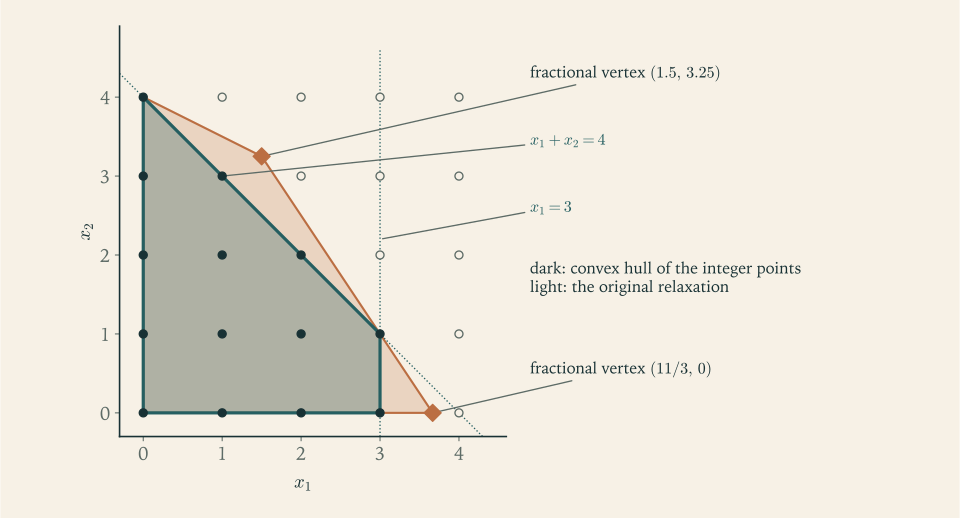
Let \(X\) be the set of fourteen feasible plans of Example 1.1 and \(P\) the original formulation, \(x_1+2x_2\le 8\) , \(3x_1+2x_2\le 11\) , \(x\ge 0\) . Two further inequalities hold at every point of \(X\) . Since \(3x_1\le 11\) forces the integer \(x_1\) to be at most \(3\) , we have \(x_1\le 3\) . And no feasible plan carries more than four pallets in total, as the list in Example 1.1 shows, so \(x_1+x_2\le 4\) . Let \(P'\) be \(P\) with the inequality \(x_1\le 3\) added, and \(P''\) be \(P\) with both added. All three are formulations for \(X\) , and \(P''\subseteq P'\subseteq P\) .
For the profit objective \(5x_1+4x_2\) the three relaxations give
The inequality \(x_1\le 3\) is valid and makes the formulation stronger, yet it does not improve this bound, because the fractional optimum \((1.5,3.25)\) satisfies it. The inequality \(x_1+x_2\le 4\) is violated by that point, since \(1.5+3.25=4.75\) , and adding it moves the relaxation optimum to \((3,1)\) , which is an integer point. For \(P''\) the relaxation solves the problem.
Change the objective to \(x_1\) alone and the roles reverse: \(z_{LP}(P)=11/3\) , attained at the fractional vertex \((11/3,0)\) , while \(z_{LP}(P')=3\) . Which inequality helps depends on where the objective points. A formulation that is good for every objective must exclude every fractional vertex.
5.2 The convex hull is the best description
Definition 5.3 (convex hull). The convex hull of a finite set \(X=\{x^1,\dots,x^K\}\subseteq\mathbb R^n\) is the set of all convex combinations of its points,
Theorem 5.4 (optimizing over the hull). Let \(X\subseteq\mathbb Z^n\) be finite and nonempty. Then (a) every formulation \(P\) for \(X\) contains \(\operatorname{conv}(X)\) ; (b) for every \(c\in\mathbb R^n\) , \(\max\{c^{\top}x:x\in X\}=\max\{c^{\top}x:x\in\operatorname{conv}(X)\}\) ; and (c) every extreme point of \(\operatorname{conv}(X)\) belongs to \(X\) .
Proof. (a) A polyhedron is convex and \(P\) contains each point of \(X\) , so it contains all their convex combinations.
(b) The right side is at least the left because \(X\subseteq\operatorname{conv}(X)\) . Conversely, for \(x=\sum_k\lambda_kx^k\) in the hull, \(c^{\top}x=\sum_k\lambda_kc^{\top}x^k\le\max_kc^{\top}x^k\) , since a weighted average does not exceed the largest of the averaged numbers.
(c) Let \(x=\sum_k\lambda_kx^k\) be an extreme point of the hull, written with distinct points and positive weights. If there is only one term, \(x\in X\) . Otherwise \(0<\lambda_1<1\) , and \(x=\lambda_1x^1+(1-\lambda_1)y\) where \(y=\sum_{k\ge 2}\lambda_kx^k/(1-\lambda_1)\) belongs to the hull. If \(y=x^1\) then \(x=x^1\in X\) . If \(y\ne x^1\) , put \(\varepsilon=\min\{\lambda_1,1-\lambda_1\}\) ; the two points \(x\pm\varepsilon(x^1-y)\) lie on the segment from \(y\) to \(x^1\) , are different from each other, and have midpoint \(x\) , which contradicts the definition of an extreme point.
The hull of a finite set is a polytope: it can be described by finitely many linear inequalities. That is one half of the Minkowski–Weyl theorem of polyhedral theory, which we use without proof. For the cargo set the description is short.
Definition 5.5 (ideal formulation). A formulation \(P\) for \(X\) is ideal if \(P=\operatorname{conv}(X)\) .
By Theorem 5.4 an ideal formulation is at least as strong as every other, and its relaxation solves the integer problem for every objective: a linear program over a polytope has an optimal vertex, a theorem of Continuous Optimization, and the vertices of the hull are points of \(X\) . With an ideal formulation in hand, integer programming is linear programming.
For the cargo set, \(P''\) is ideal: its vertices are \((0,0)\) , \((3,0)\) , \((3,1)\) , and \((0,4)\) , all in \(X\) , and every point of \(X\) satisfies its inequalities. Notice what happened to the original constraints. Neither \(x_1+2x_2\le 8\) nor \(3x_1+2x_2\le 11\) is needed any longer: the hull is described by \(x_1\le 3\) , \(x_1+x_2\le 4\) , and nonnegativity. The inequalities of an ideal formulation need not resemble those of the model one first writes down.
Why not always use the ideal formulation? Because for most problems it cannot be written down. The hull of the tours of the symmetric travelling salesman problem on even ten cities has more than fifty billion facets, and for NP-hard problems in general no manageable description of the hull is to be expected. The ideal formulation is a direction to move in. The problems of Chapters 2 to 4 are those for which the natural formulation is already ideal, and Chapter 6 explains how to recognize that.
Common mistake. Judging a formulation by its size. Fewer constraints make each linear program faster to solve and can make the integer program far slower, because a weaker relaxation leaves more for the search to do. The next section gives an instance in which adding nine constraints raises the bound from \(11\) to the optimal value. The right comparison is by inclusion of the relaxations.
5.3 Strength in practice: where to put the linking constraints
In the uncapacitated facility location problem there are \(m\) candidate facilities and \(n\) clients. Opening facility \(i\) costs \(f_i\) , and serving client \(j\) from facility \(i\) costs \(c_{ij}\) . Every client must be served from an open facility, at minimum total cost. Let \(y_i\in\{0,1\}\) say whether facility \(i\) is open and \(x_{ij}\ge 0\) be the fraction of client \(j\) served from \(i\) . Both of the following models minimize \(\sum_if_iy_i+\sum_{i,j}c_{ij}x_{ij}\) subject to \(\sum_ix_{ij}=1\) for every client. They differ in how they say “no service from a closed facility”:
Proposition 5.6 (disaggregation is stronger). With \(y\) binary, the two sets of linking constraints admit the same solutions. With \(0\le y\le 1\) , every point satisfying the disaggregated constraints satisfies the aggregated ones, and the converse is false whenever \(n\ge 2\) .
Proof. If \(y_i=0\) , both versions force \(x_{ij}=0\) for all \(j\) . If \(y_i=1\) , the disaggregated version says \(x_{ij}\le 1\) , which already follows from \(\sum_ix_{ij}=1\) and \(x\ge 0\) , and the aggregated version says \(\sum_jx_{ij}\le n\) , which follows as well. So the binary solutions agree. For fractional \(y\) , adding the \(n\) inequalities \(x_{ij}\le y_i\) over \(j\) gives the aggregated inequality. For the converse, let \(x_{i1}=1\) , \(x_{ij}=0\) for \(j\ge 2\) , and \(y_i=1/n\) : the aggregated constraint holds with equality, and \(x_{i1}\le y_i\) fails.
The aggregated relaxation lets a facility serve one client completely while being only \(1/n\) open. It pays one \(n\) -th of the fixed cost per client served, as if facilities could be rented by the slice.
Example 5.2: Three warehouses, four customers
Each of three warehouses costs \(6\) to open, and the service costs are
with rows for warehouses and columns for customers.
The integer optimum. With one warehouse open the totals are \(6+14=20\) , \(6+12=18\) , and \(6+15=21\) . With two open, each customer uses the cheaper: warehouses 1 and 2 give \(12+8=20\) , 1 and 3 give \(12+7=19\) , 2 and 3 give \(12+9=21\) . With all three open the total is \(18+5=23\) . The optimum is \(18\) : open warehouse 2 alone.
The aggregated relaxation. Here \(n=4\) , and it is optimal to set \(y_i=\tfrac14\sum_jx_{ij}\) , so serving a customer from warehouse \(i\) costs \(c_{ij}+6/4\) whichever warehouse is used. Each customer takes its cheapest service: costs \(1,2,1,1\) , from warehouses 1, 1, 2, 3. The bound is \(5+4\cdot 1.5=11\) , with \(y=(\tfrac12,\tfrac14,\tfrac14)\) : the relaxation pays the fixed cost of one warehouse in total and enjoys the service costs of having all three open.
The disaggregated relaxation. Its optimal value is \(18\) , attained at the integer solution itself. To see that nothing fractional does better, use duality: assign each customer \(j\) a price \(v_j\) and require that for each warehouse the total excess \(\sum_j\max\{v_j-c_{ij},0\}\) not exceed the opening cost \(6\) ; then \(\sum_jv_j\) is a lower bound on the relaxation. Indeed, writing \(e_{ij}=\max\{v_j-c_{ij},0\}\) , any feasible point has \(f_iy_i\ge\sum_je_{ij}y_i\ge\sum_je_{ij}x_{ij}\) , so its cost is at least \(\sum_{i,j}(c_{ij}+e_{ij})x_{ij}\ge\sum_{i,j}v_jx_{ij}=\sum_jv_j\) . The prices \(v=(5,4,4,5)\) give excesses \(4+2+0+0=6\) , \(0+2+3+1=6\) , and \(0+0+1+4=5\) , all within \(6\) , and \(5+4+4+5=18\) .
The two formulations have the same integer solutions, three constraints against twelve, and bounds of \(11\) and \(18\) for an optimum of \(18\) . This is the pair of models from the chapter opening.
The disaggregated formulation is not ideal in general. With three warehouses of opening cost \(2\) and three customers, each of whom can be served at zero cost from two of the warehouses in a cyclic pattern and at prohibitive cost from the third, the disaggregated relaxation opens every warehouse halfway for a bound of \(3\) , while any integer solution must open two, at cost \(4\) . Exercise 6 works this out.
5.4 The price of a large constant
The device \(y\le Mx\) of Chapter 1 is the commonest source of weak formulations, because the relaxation satisfies it with \(x=y/M\) , and the larger \(M\) is, the less of the fixed cost the relaxation pays.
Example 5.3: One constraint, three constants
A plant can make a product at a fixed cost of \(100\) for a production run plus \(2\) per unit, or buy it at \(5\) per unit; \(30\) units are needed. With \(x\in\{0,1\}\) for the run, \(y\) for the quantity made and \(w\) for the quantity bought, the model is
Making all \(30\) units costs \(100+60=160\) and buying them costs \(150\) , so the optimum is \(150\) : buy.
In the relaxation each unit made costs \(2+100/M\) , since \(x=y/M\) is the cheapest way to permit \(y\) . With \(M=1000\) , a constant chosen “to be safe”, a unit made costs \(2.1\) , the relaxation makes everything, and the bound is \(63\) . With \(M=40\) , the plant’s capacity, a unit made costs \(4.5\) , still below \(5\) ; the relaxation makes everything with \(x=0.75\) and the bound is \(135\) . With \(M=30\) , the most that could ever be needed, a unit made costs \(2+100/30\approx 5.33\) , more than buying; the relaxation buys everything and the bound is \(150\) , the true optimum.
All three constants are valid. They give bounds of \(63\) , \(135\) , and \(150\) . The smallest valid constant, the tightest bound on \(y\) that the rest of the model implies, turned a formulation that needs search into one that needs none.
Common mistake. Choosing \(M\) too small in order to be strong. The constant must not cut off any feasible integer solution. In Example 5.3, \(M=20\) would forbid making all \(30\) units, which is a legitimate plan, and if the purchase price were \(6\) it would exclude the optimum. Compute \(M\) as a bound implied by the other constraints, here \(y\le 30\) from \(y+w=30\) and \(w\ge 0\) , and then no smaller.
5.5 Cliques, products, and tours
Three more modelling situations show the same phenomenon in different dress.
Conflicts. In the independent set problem of Chapter 1 the edge formulation has a constraint \(x_v+x_w\le 1\) for each edge. If \(K\) is a clique, at most one of its nodes can be chosen, so the clique inequality \(x(K)\le 1\) is valid. It implies the edge inequality for every edge inside \(K\) and is not implied by them when \(K\) has three or more nodes: the point with every coordinate \(\tfrac12\) satisfies all edge inequalities and gives \(x(K)=\lvert K\rvert/2\) .
Example 5.4: Edge inequalities against clique inequalities
Take the graph of Example 1.5: triangles on \(\{1,2,3\}\) and \(\{4,5,6\}\) joined by the edges \(24\) and \(35\) . Its largest independent set has two nodes.
The edge formulation has eight constraints. Setting every variable to \(\tfrac12\) satisfies all of them and gives objective value \(3\) . No point of the relaxation does better, since adding the three edge constraints of each triangle gives \(2(x_1+x_2+x_3)\le 3\) and \(2(x_4+x_5+x_6)\le 3\) . So the edge relaxation has \(z_{LP}=3\) , and even after rounding down it does not prove that \(2\) is optimal.
The clique formulation replaces the six triangle edges by \(x_1+x_2+x_3\le 1\) and \(x_4+x_5+x_6\le 1\) and keeps \(x_2+x_4\le 1\) and \(x_3+x_5\le 1\) . Adding the two clique inequalities gives \(x_1+\dots+x_6\le 2\) at once, so \(z_{LP}=2=z^\star\) . Four constraints do better than eight, which is a reminder that strength and size are unrelated in both directions.
Products. A cost that is incurred only when two options are both chosen involves the product \(x_1x_2\) of two binary variables, which is not linear.
Proposition 5.7 (linearizing a product of binaries). For \(x_1,x_2\in\{0,1\}\) , a real number \(z\) satisfies
if and only if \(z=x_1x_2\) .
Proof. If \(x_1=x_2=1\) the constraints read \(z\le 1\) and \(z\ge 1\) , so \(z=1\) . Otherwise some \(x_i=0\) , and the constraints \(z\le x_i\) and \(z\ge 0\) give \(z=0\) , while \(z\ge x_1+x_2-1\) holds because its right side is at most \(0\) . In both cases \(z\) equals the product, and conversely the product satisfies all four constraints.
Tours. For the travelling salesman problem on \(n\) cities with arc variables \(x_{ij}\in\{0,1\}\) , the constraints that each city is left once and entered once describe assignments, which may break into several small cycles, or subtours. Two classical ways of excluding them are the subtour elimination constraints, which for each set \(S\) of cities with \(2\le\lvert S\rvert\le n-2\) require at least one chosen arc from \(S\) to its complement, and the Miller–Tucker–Zemlin constraints, which introduce an order variable \(t_i\) for each city other than the first and require \(t_i-t_j+(n-1)x_{ij}\le n-2\) for all pairs of those cities. The first family has exponentially many members; the second has about \(n^2\) . The second is built on a large constant.
Example 5.5: A compact formulation that is weak
Six cities lie in two clusters, at \((0,0)\) , \((1,0)\) , \((0,1)\) and at \((10,0)\) , \((11,0)\) , \((10,1)\) , with distances measured along the grid. Within a cluster the three distances are \(1\) , \(1\) , and \(2\) . A tour must cross between the clusters twice, and the best tour has length \(24\) .
With only the assignment constraints, the relaxation’s optimum is two triangles, one in each cluster, of total length \(4+4=8\) . Adding the Miller–Tucker–Zemlin constraints does not change the bound: putting weight \(\tfrac12\) on each of the two orientations of each triangle satisfies them, with all order variables equal, since \(t_i-t_j+5\cdot\tfrac12\le 4\) holds when \(t_i=t_j\) . The bound stays at \(8\) . Adding the subtour elimination constraints instead, fifty of them for six cities, forces at least one unit of flow out of each cluster, and the bound becomes \(24\) , the length of the optimal tour.
The same integer solutions, and bounds of \(8\) and \(24\) . A solver given the compact formulation must discover by search what the subtour constraints state directly. Chapter 8 shows that the exponential family is usable in practice, because a violated member can be found by a minimum-cut computation and added only when needed.
5.6 Measuring what is left
Definition 5.8 (integrality gap). For a maximization instance with formulation \(P\) , the absolute gap is \(z_{LP}(P)-z^\star\) , and when \(z^\star>0\) the relative gap is the ratio \(z_{LP}(P)/z^\star\) . For a minimization instance the absolute gap is \(z^\star-z_{LP}(P)\) and the relative gap is \(z^\star/z_{LP}(P)\) . The integrality gap of a formulation for a problem is the supremum of the relative gap over all instances.
In this chapter’s examples the relative gaps were \(20.5/19\) for the cargo problem, \(18/11\) and \(1\) for the two location models, \(150/63\) , \(150/135\) , and \(1\) for the three constants, \(3/2\) and \(1\) for the two independent set models, and \(3\) and \(1\) for the two tour models. A relative gap of \(1\) on an instance means the relaxation proved optimality on that instance; an integrality gap of \(1\) for a formulation means it does so on every instance, which is the ideal case.
The gap matters twice over. For exact methods it measures the work left for branching and cutting. For approximation it bounds what rounding can achieve: Chapter 10 obtains a vertex cover of at most twice the minimum size by rounding the relaxation, and no rounding analysis that compares only with the relaxation can do better, because the integrality gap of that relaxation approaches \(2\) (Exercise 16).
A final caution about what this chapter has and has not shown. Strength is a property of a formulation and an objective together; Example 5.1 showed one inequality that helps for one objective and not another. And strength has a cost: the twelve-constraint location model has four times the rows of the three-constraint one, and on large instances that ratio is the number of clients. The art lies in finding inequalities that are strong where the objective looks, and the systematic way of doing that, adding them only when the relaxation’s solution violates them, is the subject of Chapter 8.
Exercises
-
Let \(X=\{(0,0),(1,0),(0,1),(1,1),(2,0)\}\) . For each polyhedron decide whether it is a formulation for \(X\) , justifying by naming an integer point wrongly included or excluded where it is not: (a) \(x\ge 0\) , \(x_1+x_2\le 2\) , \(x_2\le 1\) ; (b) \(x\ge 0\) , \(x_1+2x_2\le 3\) ; (c) \(x\ge 0\) , \(3x_1+2x_2\le 6\) , \(x_2\le 1\) .
Answer
(a) Yes: the integer points with \(x_2\le 1\) and \(x_1+x_2\le 2\) are \((0,0)\) , \((1,0)\) , \((2,0)\) , \((0,1)\) , \((1,1)\) . (b) No: \((3,0)\) satisfies \(x_1+2x_2\le 3\) and is not in \(X\) . (c) Yes: \(3x_1+2x_2\le 6\) allows \(x_1\le 2\) when \(x_2=0\) and \(x_1\le 1\) when \(x_2=1\) , and \(x_2\le 1\) excludes the rest. Formulation (a) is stronger than (c): its vertices \((0,0)\) , \((2,0)\) , \((1,1)\) , \((0,1)\) all satisfy \(3x_1+2x_2\le 6\) , so (a) is contained in (c), while the vertex \((4/3,1)\) of (c) violates \(x_1+x_2\le 2\) . Since all four vertices of (a) belong to \(X\) , (a) is the convex hull of \(X\) .
-
The inequalities \(2x_1+2x_2+2x_3\le 3\) and \(x_1+x_2+x_3\le 1\) , each together with \(0\le x\le 1\) , define two polyhedra. Show that they contain the same binary points, decide which is stronger, and compute both relaxation bounds for the objective \(x_1+x_2+x_3\) .
Solution
Same binary points. For a binary vector the sum \(x_1+x_2+x_3\) is an integer. The first inequality says the sum is at most \(3/2\) , which for an integer means at most \(1\) ; the second says at most \(1\) . So both polyhedra contain exactly the binary vectors with at most one coordinate equal to one: \((0,0,0)\) , \((1,0,0)\) , \((0,1,0)\) , \((0,0,1)\) .
Strength. Call the polyhedra \(P_1\) , from \(2x_1+2x_2+2x_3\le 3\) , and \(P_2\) , from \(x_1+x_2+x_3\le 1\) . If \(x\in P_2\) then \(2(x_1+x_2+x_3)\le 2\le 3\) , so \(x\in P_1\) ; thus \(P_2\subseteq P_1\) . The point \((\tfrac12,\tfrac12,\tfrac12)\) has sum \(\tfrac32\) , so it belongs to \(P_1\) and not to \(P_2\) . The inclusion is strict and \(P_2\) is the stronger formulation.
Bounds. Over \(P_1\) the objective \(x_1+x_2+x_3\) is at most \(\tfrac32\) , attained at \((\tfrac12,\tfrac12,\tfrac12)\) , so \(z_{LP}(P_1)=\tfrac32\) . Over \(P_2\) it is at most \(1\) , attained at \((1,0,0)\) , so \(z_{LP}(P_2)=1=z^\star\) . Dividing the first inequality by \(2\) and rounding the right side down turns it into the second, the simplest instance of the rounding procedure of Chapter 8.
-
Let \(X\) be the set of integer points satisfying \(-x_1+2x_2\le 4\) , \(5x_1+2x_2\le 20\) , and \(x\ge 0\) . List \(X\) column by column, find the vertices of \(\operatorname{conv}(X)\) , give an inequality description of the hull, and compare \(z_{LP}\) and \(z^\star\) for the objective \(x_1+x_2\) .
Solution
For \(x_1=0\) the first constraint gives \(x_2\le 2\) . For \(x_1=1\) : \(2x_2\le 5\) and \(2x_2\le 15\) , so \(x_2\le 2\) . For \(x_1=2\) : \(2x_2\le 6\) and \(2x_2\le 10\) , so \(x_2\le 3\) . For \(x_1=3\) : \(2x_2\le 7\) and \(2x_2\le 5\) , so \(x_2\le 2\) . For \(x_1=4\) : \(2x_2\le 0\) . So \(X\) has \(3+3+4+3+1=14\) points.
The topmost points of the columns are \((0,2)\) , \((1,2)\) , \((2,3)\) , \((3,2)\) , \((4,0)\) . The point \((1,2)\) lies below the segment from \((0,2)\) to \((2,3)\) , which passes through \((1,2.5)\) , so it is not a vertex. The vertices of the hull are \((0,0)\) , \((4,0)\) , \((3,2)\) , \((2,3)\) , \((0,2)\) .
The edges give the inequalities. Through \((0,2)\) and \((2,3)\) : \(-x_1+2x_2\le 4\) , one of the original constraints. Through \((2,3)\) and \((3,2)\) : \(x_1+x_2\le 5\) . Through \((3,2)\) and \((4,0)\) : \(2x_1+x_2\le 8\) . With \(x\ge 0\) these describe the hull:
\[ \operatorname{conv}(X)=\{x\ge 0:\ -x_1+2x_2\le 4,\ x_1+x_2\le 5,\ 2x_1+x_2\le 8\}. \]For the objective \(x_1+x_2\) the original relaxation is maximized where both original constraints are active: subtracting them gives \(6x_1=16\) , so \(x=(8/3,10/3)\) and \(z_{LP}=6\) . Over the hull the maximum is \(z^\star=5\) , attained at \((2,3)\) and \((3,2)\) . The original constraint \(5x_1+2x_2\le 20\) does not appear in the hull at all.
-
Prove that if \(P_1\) and \(P_2\) are formulations for the same set \(X\) then \(P_1\cap P_2\) is a formulation for \(X\) that is at least as strong as each, and give an example with \(n=2\) in which neither of \(P_1\) , \(P_2\) contains the other.
Solution
Since \(P_1\cap\mathbb Z^n=X\) and \(P_2\cap\mathbb Z^n=X\) , we have \((P_1\cap P_2)\cap\mathbb Z^n=(P_1\cap\mathbb Z^n)\cap(P_2\cap\mathbb Z^n)=X\) . The intersection of two polyhedra is a polyhedron: take the inequalities of both together. So \(P_1\cap P_2\) is a formulation for \(X\) . It is contained in \(P_1\) and in \(P_2\) , so by Proposition 5.2 it is at least as strong as each, and its bound is at most the smaller of theirs for every objective.
For the example let \(X=\{(0,0),(1,0),(0,1),(1,1)\}\) , and take
\[ P_1=\{0\le x_1\le\tfrac32,\ 0\le x_2\le 1\},\qquad P_2=\{0\le x_1\le 1,\ 0\le x_2\le\tfrac32\}. \]Each contains the four points of \(X\) and no other integer point. The point \((\tfrac32,0)\) lies in \(P_1\) only and \((0,\tfrac32)\) in \(P_2\) only, so neither contains the other. Their intersection is the unit square, which is the convex hull of \(X\) and hence ideal. For the objective \(x_1\) the bounds are \(\tfrac32\) and \(1\) ; for the objective \(x_2\) they are \(1\) and \(\tfrac32\) : each formulation is better for one objective.
-
Two facilities have opening costs \(4\) and \(5\) , and three clients have service costs \((1,3,6)\) from the first and \((5,2,1)\) from the second. Compute the integer optimum by enumeration, the aggregated relaxation bound by the per-client argument of Example 5.2, and verify that the prices \(v=(5,3,5)\) certify the disaggregated bound in the manner of Example 5.2.
Solution
Integer optimum. Facility 1 alone: \(4+(1+3+6)=14\) . Facility 2 alone: \(5+(5+2+1)=13\) . Both: \(9+(1+2+1)=13\) . The optimum is \(13\) , attained twice.
Aggregated bound. With \(n=3\) clients, serving a client from facility \(i\) costs \(c_{ij}+f_i/3\) in the relaxation. From facility 1 the three costs are \(1+\tfrac43\) , \(3+\tfrac43\) , \(6+\tfrac43\) ; from facility 2 they are \(5+\tfrac53\) , \(2+\tfrac53\) , \(1+\tfrac53\) . Client 1 prefers facility 1 at \(\tfrac73\) ; client 2 prefers facility 2 at \(\tfrac{11}3\) against \(\tfrac{13}3\) ; client 3 prefers facility 2 at \(\tfrac83\) . The bound is \(\tfrac73+\tfrac{11}3+\tfrac83=\tfrac{26}3\approx 8.67\) , with \(y=(\tfrac13,\tfrac23)\) .
Disaggregated bound. With prices \(v=(5,3,5)\) the excess at facility 1 is \(\max\{5-1,0\}+\max\{3-3,0\}+\max\{5-6,0\}=4\) , which does not exceed its opening cost \(4\) . At facility 2 it is \(\max\{5-5,0\}+\max\{3-2,0\}+\max\{5-1,0\}=5\) , which does not exceed \(5\) . So the prices are feasible and every point of the disaggregated relaxation costs at least \(5+3+5=13\) . The integer solution costs \(13\) , so the disaggregated relaxation has value exactly \(13\) and proves optimality, while the aggregated one leaves a gap of more than \(4\) .
-
Three facilities each cost \(2\) to open. Client 1 can be served at cost \(0\) from facilities 1 and 3, client 2 from facilities 1 and 2, client 3 from facilities 2 and 3, and at cost \(10\) otherwise. Show that \(y=(\tfrac12,\tfrac12,\tfrac12)\) with each client split equally between its two free facilities is feasible for the disaggregated relaxation with cost \(3\) , and that the integer optimum is \(4\) .
Solution
Feasibility. Each client is split equally between its two free facilities, so \(\sum_ix_{ij}=\tfrac12+\tfrac12=1\) for each client. Every positive \(x_{ij}\) equals \(\tfrac12=y_i\) , so \(x_{ij}\le y_i\) holds everywhere. The service cost is zero and the opening cost is \(2\cdot\tfrac32=3\) .
Integer optimum. One open facility is free for only two of the three clients: facility 1 serves clients 1 and 2 at zero cost, and client 3 would cost \(10\) . So one facility costs \(2+10=12\) . Two open facilities cover all three clients at zero service cost, since every client is free at two of the three facilities and so at one of any two; the cost is \(4\) . Three facilities cost \(6\) . The optimum is \(4\) .
Why the relaxation cannot do better than \(3\) . Prices \(v=(1,1,1)\) give each facility an excess of \(1+1+0=2\) , within its opening cost, so \(3\) is a lower bound and the fractional point is optimal. The relaxation value \(3\) is strictly below \(4\) : the disaggregated formulation is strong and still not ideal. The structure responsible is an odd cycle, clients and facilities alternating around a hexagon in which each “open” decision is shared by two clients, the same structure as the triangle of Section 4.6.
-
A model contains \(y_1+y_2\le 50\) , \(0\le y_1\le 35\) , \(0\le y_2\le 40\) , and the switching constraint \(y_1+2y_2\le M x\) with \(x\) binary. Find the smallest valid value of \(M\) by maximizing the left side over the other constraints, and say what goes wrong with \(M=100\) .
Solution
The constant \(M\) must be at least the largest value that \(y_1+2y_2\) can take when the switch is on, that is, the maximum of \(y_1+2y_2\) over \(y_1+y_2\le 50\) , \(0\le y_1\le 35\) , \(0\le y_2\le 40\) . The variable \(y_2\) has the larger coefficient, so make it as large as possible: \(y_2=40\) . Then \(y_1\le 10\) from the joint constraint, and \(y_1=10\) . The maximum is \(10+80=90\) . A check of the other vertex, \(y_1=35\) , \(y_2=15\) , gives \(65\) .
So the smallest valid constant is \(M=90\) . Any smaller value would cut off the feasible plan \((10,40)\) when \(x=1\) .
With \(M=100\) the model is still correct for binary \(x\) , but the relaxation is weaker: a fractional \(x\) now needs only \(x\ge(y_1+2y_2)/100\) where the tight model needs \(x\ge(y_1+2y_2)/90\) , so less of any fixed cost attached to \(x\) is charged and the bound drops. Adding the bounds \(y_1\le 35x\) and \(y_2\le 40x\) as separate constraints would strengthen the model further, as in Proposition 5.6.
-
Extend Proposition 5.7 to a product of three binary variables: give a set of linear constraints forcing \(z=x_1x_2x_3\) and prove that it works.
Solution
Use the constraints
\[ z\le x_1,\qquad z\le x_2,\qquad z\le x_3,\qquad z\ge x_1+x_2+x_3-2,\qquad z\ge 0 . \]Let \(x_1,x_2,x_3\in\{0,1\}\) . If all three equal \(1\) , the first three constraints give \(z\le 1\) and the fourth gives \(z\ge 1\) , so \(z=1=x_1x_2x_3\) . Otherwise some \(x_i=0\) ; then \(z\le x_i=0\) and \(z\ge 0\) give \(z=0=x_1x_2x_3\) , and the fourth constraint holds because \(x_1+x_2+x_3-2\le 0\) when at most two of the variables are one. Conversely, in both cases the value \(z=x_1x_2x_3\) satisfies all five constraints, as the same case check shows. So for binary \(x\) the constraints hold exactly when \(z\) is the product.
The pattern extends to \(k\) variables with \(z\le x_i\) for each \(i\) and \(z\ge\sum_ix_i-(k-1)\) . Note that \(z\) itself need not be declared binary: the constraints force it to \(0\) or \(1\) once the \(x_i\) are binary.
-
Four constraints \(a_k^{\top}y\le\beta_k\) , \(k=1,\dots,4\) , are given, and at least two of them must hold. Formulate this with binary variables and constants \(M_k\) , and state precisely what each \(M_k\) must bound.
Hint
Introduce \(\delta_k\in\{0,1\}\) with \(\delta_k=1\) meaning constraint \(k\) is enforced: \(a_k^{\top}y\le\beta_k+M_k(1-\delta_k)\) and \(\delta_1+\delta_2+\delta_3+\delta_4\ge 2\) . Each \(M_k\) must be an upper bound on \(a_k^{\top}y-\beta_k\) over all \(y\) that are otherwise feasible, and should be the smallest such bound.
-
A variable \(w\) must take one of the values \(0\) , \(3\) , \(5\) , or \(9\) . Write this requirement with binary variables and linear constraints, and explain why \(w\in\{0,1,\dots,9\}\) with integrality is not an acceptable substitute.
Answer
\(w=3\delta_1+5\delta_2+9\delta_3\) with \(\delta_1+\delta_2+\delta_3\le 1\) and \(\delta_k\in\{0,1\}\) . Requiring only that \(w\) be an integer between \(0\) and \(9\) would admit the values \(1,2,4,6,7,8\) , which are not allowed: it is a different set, not a weaker description of the same one.
-
Explain what is wrong with this reasoning: “Formulation A has \(20\) constraints and formulation B has \(200\) constraints for the same integer set, so A will solve faster because each of its linear programs is smaller.”
Hint
The number of constraints affects the time per linear program. The total time is that multiplied by the number of linear programs the search must solve, which depends on how close the relaxation bound is to the optimum. Compare the two location models of Example 5.2: three constraints with bound \(11\) , twelve with bound \(18\) .
-
For the complete graph on four nodes, compute the relaxation bound of the edge formulation of the independent set problem and of the formulation with the single clique inequality on all four nodes, and state the integer optimum.
Answer
Edge formulation: every variable \(\tfrac12\) is feasible with value \(2\) , and adding the six edge constraints gives \(3x(V)\le 6\) , so \(z_{LP}=2\) . With the clique inequality \(x_1+x_2+x_3+x_4\le 1\) , \(z_{LP}=1\) . The integer optimum is \(1\) .
-
In a knapsack constraint \(\sum_ja_jx_j\le b\) with binary variables and positive integer weights, show that if \(a_i+a_k>b\) then \(x_i+x_k\le 1\) is valid, and that if some \(a_i>b\) then \(x_i=0\) in every feasible solution; apply both observations to \(6x_1+5x_2+4x_3+9x_4\le 8\) .
Solution
First claim. Suppose \(a_i+a_k>b\) and some feasible binary \(x\) had \(x_i=x_k=1\) . All weights are positive and all variables nonnegative, so \(\sum_ja_jx_j\ge a_i+a_k>b\) , contradicting feasibility. Hence no feasible solution has both, which is the inequality \(x_i+x_k\le 1\) .
Second claim. If \(a_i>b\) and \(x_i=1\) then \(\sum_ja_jx_j\ge a_i>b\) . So \(x_i=0\) in every feasible solution.
Application. In \(6x_1+5x_2+4x_3+9x_4\le 8\) , the weight \(9\) exceeds \(8\) , so \(x_4=0\) . Among the other three, \(6+5=11\) , \(6+4=10\) , and \(5+4=9\) all exceed \(8\) , so \(x_1+x_2\le 1\) , \(x_1+x_3\le 1\) , and \(x_2+x_3\le 1\) . The three variables are pairwise in conflict, a clique, so the single inequality \(x_1+x_2+x_3\le 1\) is valid and implies all three. The feasible set is: at most one of the first three items, and never the fourth. The formulation \(x_1+x_2+x_3\le 1\) , \(x_4=0\) , \(0\le x\le 1\) is ideal, whereas the original constraint admits fractional points such as \((1,\tfrac25,0,0)\) .
-
Use Theorem 4.11 to explain why the constraints of the assignment problem, with \(0\le x_{ij}\le 1\) in place of the binary requirement, are an ideal formulation for the set of permutation matrices.
Hint
Theorem 4.11 says every point of the polyhedron of doubly stochastic matrices is a convex combination of permutation matrices, so the polyhedron is contained in their convex hull; Theorem 5.4(a) gives the reverse inclusion. Hence the two sets are equal and the formulation is ideal by Definition 5.5.
-
The path linear program of Section 2.5 has an integral optimal solution for every nonnegative length vector, by Proposition 2.6. Explain why this alone does not show that its feasible region is the convex hull of the path vectors, and name what else lies in the region.
Hint
The feasible region also contains flows that are not paths: a path plus any nonnegative amount of flow around a cycle is feasible, so the region is unbounded when the network has a cycle, while the hull of finitely many path vectors is bounded. Proposition 2.6 says that minimizing a nonnegative objective never benefits from the extra points; it does not say they are absent.
-
For the complete graph on \(n\) nodes, the vertex cover problem minimizes \(x(V)\) subject to \(x_v+x_w\ge 1\) on every edge. Show that the relaxation has value at most \(n/2\) , that the integer optimum is \(n-1\) , and that the relative gap tends to \(2\) .
Solution
Relaxation. The point with every \(x_v=\tfrac12\) satisfies \(x_v+x_w=1\ge 1\) on every edge, so it is feasible, with objective \(n/2\) . Hence \(z_{LP}\le n/2\) . In fact equality holds for \(n\ge 3\) : adding the constraints over all \(n(n-1)/2\) edges, each variable appears \(n-1\) times, giving \((n-1)x(V)\ge n(n-1)/2\) .
Integer optimum. If two nodes \(v\) and \(w\) were both left out of a cover, the edge \(vw\) , which exists in a complete graph, would be uncovered. So a cover omits at most one node and has at least \(n-1\) nodes; and any \(n-1\) nodes do form a cover. Thus \(z^\star=n-1\) .
Gap. For this minimization problem the relative gap is
\[ \frac{z^\star}{z_{LP}}=\frac{n-1}{n/2}=2-\frac2n , \]which increases to \(2\) as \(n\) grows. So the integrality gap of the edge formulation of vertex cover is at least \(2\) , and since Chapter 10 shows that rounding always produces a cover of size at most \(2z_{LP}\) , it is exactly \(2\) .
-
Count the subtour elimination constraints and the Miller–Tucker–Zemlin constraints for \(n=10\) cities using the definitions of Section 5.5, and comment on the comparison in the light of Example 5.5.
Answer
Subtour constraints: one for each set \(S\) with \(2\le\lvert S\rvert\le 8\) , that is, \(2^{10}-1-10-10-1=1002\) . Miller–Tucker–Zemlin constraints: one for each ordered pair of distinct cities other than the first, \(9\cdot 8=72\) . The compact family is fourteen times smaller, and Example 5.5 shows it can leave the bound at a third of the optimum where the large family closes the gap.
-
Classify by the definitions of Chapter 1 the task “given a formulation \(P\) and a point \(\hat x\) , decide whether \(\hat x\in P\) ” when \(P\) is given by an explicit list of inequalities, and explain why the classification is not obvious when \(P\) is given implicitly by an exponential family such as the subtour constraints.
Hint
With an explicit list, substitute \(\hat x\) into each inequality: the work is proportional to the length of the list, which is part of the input, so the task is polynomial. With an implicit family the input is only the rule and the data, for subtour constraints a list of about \(n^2\) numbers, while the family has about \(2^n\) members; testing them one by one is exponential in the input length. Whether membership can be decided in polynomial time then depends on the family: it is the separation problem of Chapter 8, solved for subtour constraints by minimum cuts.