A collector has died and her executor must sell a painting. Several dealers want it; each knows what it is worth to him, and the executor knows none of these values. She could ask for sealed bids and sell to the highest bidder at the price he bid. She could instead sell to the highest bidder at the price the second-highest bidder offered, which sounds like giving money away. She could hold an open auction with rising prices. She could announce a minimum price below which she will not sell. Which rule brings in the most money? And which gets the painting to the dealer who values it most?
The executor’s problem is not a game; it is the choice of a game. Whatever rule she picks, the dealers will respond to it strategically, and it is the equilibrium of the game she creates that determines what she earns. This is mechanism design: the engineering side of game theory, in which the rules are the unknown. Its first surprise is that the two sealed-bid rules, which induce completely different bidding, earn her exactly the same on average. Its second is that the reason has nothing to do with auctions in particular. It follows from a description of everything that any rule whatsoever can achieve when information is private.
Throughout the chapter there are \(n\) bidders and one object. Bidder \(i\) ’s value \(v_i\) is known only to bidder \(i\) . The values are independent draws from a distribution with continuous density \(f>0\) and distribution function \(F\) on an interval \([0,\omega]\) . A bidder who obtains the object with value \(v_i\) and pays \(t\) in total has payoff \(v_i-t\) ; one who does not obtain it has payoff \(-t\) . Bidders maximize expected payoff. This is the independent private values model, and it is a Bayesian game in the sense of Chapter 7 once the rules of bidding are fixed.
9.1 The second-price auction
In a second-price sealed-bid auction each bidder submits a bid; the highest bidder wins and pays the highest of the other bids; ties are broken at random. The winner’s own bid determines whether he wins and never what he pays.
Theorem 9.1 (truthful bidding is dominant). In the second-price auction with private values, bidding one’s value, \(b_i=v_i\) , is a weakly dominant strategy for every bidder.
Proof. Fix bidder \(i\) with value \(v_i\) , fix the bids of the others, and let \(m\) be the highest of them. Bidding \(v_i\) yields \(v_i-m\) if \(v_i>m\) and \(0\) if \(v_i<m\) (and \(0\) in either outcome of a tie, where \(v_i=m\) ); that is, it yields \(\max\{v_i-m,0\}\) . Now consider any other bid \(b\) . If \(b\) wins, the payoff is \(v_i-m\) ; if it loses, the payoff is \(0\) . Either way the payoff is at most \(\max\{v_i-m,0\}\) . So truthful bidding does at least as well as \(b\) against every \(m\) . It does strictly better for some \(m\) : if \(b<v_i\) , take \(m\) strictly between \(b\) and \(v_i\) , where \(b\) loses a profitable purchase; if \(b>v_i\) , take \(m\) strictly between \(v_i\) and \(b\) , where \(b\) wins at a price above the value.
The proof conditions on a single number, the highest competing bid, and never uses the distribution of values, the number of bidders, or any assumption about how the others behave. Truthful bidding is optimal even against irrational opponents. This is the strongest form of incentive that a rule can provide, and it has a practical consequence: a bidder needs to know only his own value to bid well. An open auction in which the price rises until one bidder remains has the same logic, since staying in until the price reaches one’s value is optimal and the winner pays the price at which the last rival dropped out.
Example 9.1: Outcome and revenue with truthful bids
Suppose three dealers have values \(10\) , \(7\) , and \(4\) and bid them. The dealer with value \(10\) wins and pays \(7\) , for a payoff of \(3\) ; the others get \(0\) . Could the dealer with value \(7\) do better? To win he must bid above \(10\) , and then he pays \(10\) for something worth \(7\) to him, a payoff of \(-3\) . Could the winner do better? Any bid above \(7\) wins at the same price \(7\) , and a bid below \(7\) loses the object and the surplus of \(3\) . No bidder can gain.
The seller’s revenue is the second-highest value. With \(n\) bidders whose values are independent and uniform on \([0,1]\) , the second-highest of \(n\) such values has expectation \((n-1)/(n+1)\) : for \(n=2\) this is \(E[\min\{v_1,v_2\}]=\int_0^1 y\cdot 2(1-y)\,dy=\tfrac13\) , and in general it follows by integrating against the density \(n(n-1)y^{n-2}(1-y)\) of the second-highest value. So the expected revenue is \(\tfrac13\) with two bidders, \(\tfrac12\) with three, and \(\tfrac{9}{11}\) with ten, approaching the upper end of the range of values as competition grows.
9.2 The first-price auction
In a first-price sealed-bid auction the highest bidder wins and pays his own bid. Bidding one’s value now guarantees a payoff of zero, win or lose. To earn anything a bidder must shade, bidding below his value, and the question is by how much: a lower bid means a larger gain upon winning and a smaller chance of winning. The answer depends on what the others do, so we look for a Bayes–Nash equilibrium, and by the symmetry of the model for one in which all bidders use the same increasing bidding function \(\beta\) .
A bidder wins exactly when his value is the highest. Let \(Y\) denote the highest of the other \(n-1\) values. By independence its distribution function is \(G(y)=F(y)^{n-1}\) ; write \(g=G'\) for its density.
Theorem 9.2 (first-price equilibrium). In the first-price auction with independent private values, the bidding function
used by every bidder, is a Bayes–Nash equilibrium. In words, each bidder bids the expected value of the highest rival value, conditional on that value being below his own: \(\beta(v)=E[Y\mid Y<v]\) .
Proof. The two expressions agree by integration by parts: \(\int_0^vyg(y)\,dy=vG(v)-\int_0^vG(y)\,dy\) . The function \(\beta\) is continuous and strictly increasing, because the conditional expectation of \(Y\) given \(Y<v\) rises with \(v\) . Suppose all bidders but one use \(\beta\) , and consider the remaining bidder, with value \(v\) . A bid above \(\beta(\omega)\) wins for sure, as does \(\beta(\omega)\) , and costs more, so it is not optimal. Any other bid equals \(\beta(z)\) for some \(z\in[0,\omega]\) . Bidding \(\beta(z)\) wins when \(Y<z\) , which has probability \(G(z)\) , so the expected payoff is
Differentiating in \(z\) gives \(g(z)v-zg(z)=g(z)(v-z)\) , which is positive for \(z<v\) and negative for \(z>v\) . So \(\Pi(\cdot,v)\) is maximized at \(z=v\) : the best response is to bid \(\beta(v)\) .
The derivative \(g(z)(v-z)\) is worth a second look. A bidder who behaves as if his value were slightly higher gains the extra probability \(g(z)\) of winning something worth \(v\) , and pays for it as if it were worth \(z\) . The bidding function has been arranged so that these balance exactly at \(z=v\) .
Example 9.2: Uniform values
Let the values be uniform on \([0,1]\) , so \(F(v)=v\) and \(G(y)=y^{n-1}\) . Then \(\int_0^vG(y)\,dy=v^n/n\) and
With two bidders each bids half his value; with ten, nine tenths of it. Shading decreases with competition. As a direct check for \(n=2\) : against a rival who bids \(v_2/2\) , a bid \(b\le\tfrac12\) wins with probability \(2b\) and yields \((v-b)\cdot 2b\) , which is maximized at \(b=v/2\) .
The seller’s revenue is the winning bid, \(\tfrac{n-1}{n}\) times the highest value. The highest of \(n\) uniform values has expectation \(n/(n+1)\) , so the expected revenue is
This is exactly the expected revenue of the second-price auction in Example 9.1. In the first-price auction the winner pays his own shaded bid; in the second-price auction he pays a rival’s truthful bid; and on average the two are the same.
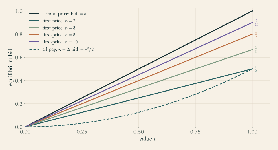
The coincidence in Example 9.2 is too exact to be an accident of the uniform distribution. Explaining it requires stepping back from particular auctions.
9.3 Mechanisms and the revelation principle
A mechanism is any set of rules for the bidders: a set of messages (bids, or anything else) for each, and a rule that turns each profile of messages into an allocation of the object and a payment by each bidder. Together with the bidders’ private values it defines a Bayesian game. The executor’s problem is to choose the mechanism, anticipating that the bidders will play an equilibrium of it. The space of mechanisms is vast, and it is not obvious how to search it. The following observation shows that one need not.
Definition 9.3 (direct mechanism). A direct mechanism asks each bidder to report a value. It is described by functions \(q_i(v)\) and \(t_i(v)\) of the profile of reports \(v=(v_1,\dots,v_n)\) : \(q_i(v)\) is the probability that bidder \(i\) receives the object and \(t_i(v)\) is bidder \(i\) ’s expected payment, with \(q_i(v)\ge 0\) and \(\sum_iq_i(v)\le 1\) . When the other bidders report truthfully, a bidder who reports \(z\) obtains the object with probability \(Q_i(z)=E[q_i(z,v_{-i})]\) and pays \(T_i(z)=E[t_i(z,v_{-i})]\) on average, the expectations being over the others’ values. The mechanism is incentive compatible if truthful reporting is a Bayes–Nash equilibrium:
It is individually rational if \(U_i(v_i)=v_iQ_i(v_i)-T_i(v_i)\ge 0\) for all \(i\) and \(v_i\) , so that every type is willing to take part.
Theorem 9.4 (revelation principle). Let \(\sigma=(\sigma_1,\dots,\sigma_n)\) be a Bayes–Nash equilibrium of any mechanism. Then there is an incentive-compatible direct mechanism that, for every profile of values, produces the same allocation probabilities and the same expected payments as the equilibrium \(\sigma\) of the original mechanism.
Proof. Define the direct mechanism as follows: on receiving the reports \((v_1,\dots,v_n)\) , compute the messages \(\sigma_1(v_1),\dots,\sigma_n(v_n)\) that the bidders would have sent in the original mechanism, and apply the original mechanism’s outcome rule to them. If all report truthfully the outcome is, by construction, that of \(\sigma\) . Suppose bidder \(i\) with value \(v_i\) could gain by reporting \(z\ne v_i\) when the others are truthful. Reporting \(z\) makes the direct mechanism play \(\sigma_i(z)\) on his behalf against the messages \(\sigma_{-i}(v_{-i})\) . Then in the original mechanism, bidder \(i\) with value \(v_i\) could gain by sending the message \(\sigma_i(z)\) in place of \(\sigma_i(v_i)\) , against the others’ equilibrium strategies. That contradicts the assumption that \(\sigma\) is an equilibrium.
The argument is almost embarrassingly short: the designer offers to play each bidder’s equilibrium strategy for him, and a bidder who trusts the machine has no reason to mislead it. Its consequence is large. Anything that can be achieved in an equilibrium of any mechanism can be achieved by a direct mechanism in which telling the truth is an equilibrium. To find out what is achievable at all, it is enough to study incentive-compatible direct mechanisms. The first-price auction, for instance, corresponds to the direct mechanism “the highest report wins and pays \(\beta\) of his report”.
The principle does not say that real mechanisms should ask for values, and it does not say that truthful reporting is the only equilibrium of the direct mechanism. It is a tool for characterizing possibilities.
Example 9.3: Incentive constraints with two types
A single buyer’s value is \(2\) or \(5\) . The seller offers a menu: a buyer who reports the low value gets the object with probability \(\tfrac12\) and pays \(1\) ; a buyer who reports the high value gets it for sure and pays \(t_H\) . For which \(t_H\) is the menu incentive compatible and individually rational?
The low type’s payoff from truth is \(2\cdot\tfrac12-1=0\) , so participation holds with nothing to spare. From misreporting it is \(2-t_H\) . Truth is optimal when \(0\ge 2-t_H\) , that is, \(t_H\ge 2\) .
The high type’s payoff from truth is \(5-t_H\) , and from claiming to be low it is \(5\cdot\tfrac12-1=1.5\) . Truth is optimal when \(5-t_H\ge 1.5\) , that is, \(t_H\le 3.5\) ; and then \(5-t_H\ge 1.5>0\) , so participation holds.
The menu works exactly for \(2\le t_H\le 3.5\) , and the seller will choose \(t_H=3.5\) . The high type cannot be charged his full value \(5\) , although he would pay it for the object, because he has the option of pretending to be the low type. He keeps a payoff of \(1.5\) that the seller cannot extract: an information rent. Its size is \((5-2)\cdot\tfrac12\) , the difference in values times the probability with which the low type is served. To reduce the rent the seller would have to serve the low type less. This trade-off between efficiency and rent is the theme of the next two sections, in continuous form.
9.4 What incentive compatibility implies
Theorem 9.5 (characterization of incentive compatibility). A direct mechanism is incentive compatible if and only if, for every bidder \(i\) : (i) the allocation probability \(Q_i\) is nondecreasing; and (ii) for every \(v_i\in[0,\omega]\) ,
Proof. Drop the index \(i\) . Since \(vQ(z)-T(z)=U(z)+(v-z)Q(z)\) , incentive compatibility says that \(U(v)\ge U(z)+(v-z)Q(z)\) for all \(v,z\) .
Necessity. Write the inequality twice, once as it stands and once with \(v\) and \(z\) exchanged:
For \(v>z\) this gives \(Q(z)\le Q(v)\) , which is (i). For (ii), divide \([0,v]\) into \(k\) equal parts by points \(0=s_0<s_1<\dots<s_k=v\) and add the inequalities for consecutive points:
The outer sums are lower and upper Riemann sums of the monotone function \(Q\)
. A monotone function on a closed interval is Riemann integrable, so both converge to \(\int_0^vQ(s)\,ds\)
as \(k\to\infty\)
(math.real-analysis.riemann-integrability).
Sufficiency. Assume (i) and (ii). Then \(U(v)-U(z)=\int_z^vQ(s)\,ds\) . If \(v>z\) , the integrand is at least \(Q(z)\) on \([z,v]\) , so the integral is at least \((v-z)Q(z)\) . If \(v<z\) , then \(U(v)-U(z)=-\int_v^zQ(s)\,ds\ge-(z-v)Q(z)=(v-z)Q(z)\) , because the integrand is at most \(Q(z)\) on \([v,z]\) . In both cases \(U(v)\ge U(z)+(v-z)Q(z)\) .
Condition (i) says that a higher value must win at least as often. Condition (ii) says that once the allocation rule is fixed, the payoff of every type is determined up to one constant: the payoff of a type \(v\) exceeds that of the lowest type by the area under \(Q\) up to \(v\) . That area is the continuous version of the information rent of Example 9.3. Since \(T=vQ-U\) , the expected payment of every type is determined as well.
Corollary 9.6 (revenue equivalence). In any incentive-compatible direct mechanism, the expected payment of bidder \(i\) with value \(v_i\) is
Consequently, any two mechanisms with equilibria that give every bidder the same allocation probabilities \(Q_i\) and give the lowest type the same payoff \(U_i(0)\) yield the same expected payment from every type of every bidder, and the same expected revenue to the seller.
Proof. The formula is (ii) of Theorem 9.5 with \(U_i=v_iQ_i-T_i\) . By the revelation principle, an equilibrium of any mechanism corresponds to an incentive-compatible direct mechanism with the same \(Q_i\) and \(T_i\) , so the formula applies to it.
This explains Example 9.2. In the symmetric equilibrium of the first-price auction and in the truthful equilibrium of the second-price auction the bidder with the highest value wins, so \(Q_i(v)=G(v)=F(v)^{n-1}\) in both; and a bidder with value \(0\) never wins and pays nothing, so \(U_i(0)=0\) in both. The corollary then says that a bidder with value \(v\) pays on average
in either format. In the first-price auction this is \(G(v)\beta(v)\) , the probability of winning times the bid, which gives back the formula of Theorem 9.2 without any differential equation. In the second-price auction it is the probability of winning times the expected second-highest value given winning. The corollary also solves auctions that have not been analysed yet.
Example 9.4: The all-pay auction
In an all-pay auction the highest bidder wins, and every bidder pays his own bid, win or lose. Lobbying contests and patent races have this structure. Suppose it has a symmetric equilibrium with an increasing bidding function \(\beta^{A}\) . Then the highest value wins and a bidder with value \(0\) bids \(0\) , so \(Q(v)=G(v)\) and \(U(0)=0\) . A bidder’s payment is his bid, with certainty, so by Corollary 9.6
For uniform values this is \(\int_0^vy(n-1)y^{n-2}\,dy=\tfrac{n-1}{n}v^n\) ; with two bidders, \(\beta^{A}(v)=v^2/2\) .
The corollary shows what an equilibrium must be if one exists; it remains to check that this is one. For \(n=2\) : if the rival bids \(v_2^2/2\) , a bidder with value \(v\) who bids \(z^2/2\) wins with probability \(z\) and pays \(z^2/2\) regardless, for an expected payoff of \(zv-z^2/2\) , which is maximized at \(z=v\) . So it is an equilibrium. A bidder with value \(\tfrac12\) bids \(\tfrac18\) , far less than the first-price bid of \(\tfrac14\) , because he pays even when he loses; the seller’s expected revenue is \(2\int_0^1\tfrac12v^2\,dv=\tfrac13\) , the same as in the other two formats.
Common mistake. Stretching these results beyond their hypotheses. Truthful bidding is dominant in the second-price auction with private values; it is not even sensible in a first-price auction, where it earns nothing, and it is not an equilibrium when values are interdependent, as Section 9.6 shows. Revenue equivalence compares equilibria that have the same allocation rule and the same payoff for the lowest type, under risk neutrality and independent values. It does not say that every auction rule earns the same. A reserve price changes who gets the object and changes revenue. Bidders with different value distributions bid asymmetrically in a first-price auction, so the highest value need not win there, while it still wins in a second-price auction; the allocations differ and so may the revenues. And risk-averse bidders shade less in a first-price auction, which then earns more. Before invoking the theorem, state the allocation rule of each equilibrium being compared.
9.5 The auction that maximizes revenue
Revenue equivalence says that the seller cannot raise expected revenue by changing the payment rule while keeping the allocation. She can raise it only by changing the allocation, and Theorem 9.5 tells her exactly what each allocation rule earns.
Proposition 9.7 (revenue as expected virtual surplus). Define the virtual value \(\psi(v)=v-\dfrac{1-F(v)}{f(v)}\) . In an incentive-compatible direct mechanism, the expected payment of bidder \(i\) is
and hence the seller’s expected revenue is \(E\bigl[\sum_i\psi(v_i)\,q_i(v)\bigr]-\sum_iU_i(0)\) .
Proof. By Corollary 9.6, \(E[T_i]=\int_0^\omega vQ_i(v)f(v)\,dv-\int_0^\omega\int_0^vQ_i(s)\,ds\,f(v)\,dv-U_i(0)\) . In the double integral exchange the order of integration over the triangle \(0\le s\le v\le\omega\) : it equals \(\int_0^\omega Q_i(s)\int_s^\omega f(v)\,dv\,ds=\int_0^\omega Q_i(s)(1-F(s))\,ds\) . Therefore
and \(E[\psi(v_i)Q_i(v_i)]=E[\psi(v_i)q_i(v)]\) by the definition of \(Q_i\) .
The virtual value is the value minus the information rent that serving this type forces the seller to leave to all higher types. The seller’s revenue is as if she collected the virtual value, not the value, of whoever gets the object.
Theorem 9.8 (optimal auction). Suppose \(\psi\) is strictly increasing, and let \(r^\star\) be the value at which \(\psi(r^\star)=0\) ; it exists and is unique because \(\psi\) is continuous with \(\psi(0)=-1/f(0)<0\) and \(\psi(\omega)=\omega>0\) . Among all incentive-compatible and individually rational mechanisms, the seller’s expected revenue is maximized by giving the object to the bidder with the highest value, provided that value is at least \(r^\star\) , and to nobody otherwise, with \(U_i(0)=0\) . A second-price auction with reserve price \(r^\star\) implements this.
Proof. By Proposition 9.7 the seller wants to maximize \(E[\sum_i\psi(v_i)q_i(v)]-\sum_iU_i(0)\) . Individual rationality requires \(U_i(0)\ge 0\) , and by Theorem 9.5(ii) it holds for all types once it holds for the lowest, so \(U_i(0)=0\) is best. For each profile \(v\) , the sum \(\sum_i\psi(v_i)q_i(v)\) with \(q_i\ge 0\) and \(\sum_iq_i\le 1\) is largest when all the probability goes to a bidder with the largest \(\psi(v_i)\) , if that is positive, and no probability is assigned if all are negative. Since \(\psi\) is increasing, the largest virtual value belongs to the largest value, and it is nonnegative exactly when that value is at least \(r^\star\) . This rule maximizes the integrand at every \(v\) , so it maximizes the expectation, provided it is incentive compatible; and it is, because under it \(Q_i(v_i)\) is \(0\) below \(r^\star\) and \(G(v_i)\) above, a nondecreasing function, so payments defined by Corollary 9.6 satisfy Theorem 9.5. In the second-price auction with reserve \(r^\star\) , bidding one’s value remains weakly dominant by the argument of Theorem 9.1, with the reserve acting as one more competing bid; the allocation is the one described, and a bidder with value \(0\) gets \(0\) .
The reserve price \(r^\star\) does not depend on the number of bidders. It is the price a seller would post when facing a single buyer: with one buyer, a posted price \(r\) earns \(r(1-F(r))\) , whose derivative \(1-F(r)-rf(r)\) vanishes exactly where \(\psi(r)=0\) .
Example 9.5: A reserve price for uniform values
For values uniform on \([0,1]\) , \(\psi(v)=v-(1-v)=2v-1\) , which is increasing, and \(r^\star=\tfrac12\) .
With one buyer, the posted price \(\tfrac12\) is accepted with probability \(\tfrac12\) and earns \(\tfrac14\) .
With two bidders and a reserve \(r\) in a second-price auction, the seller receives \(r\) if exactly one value exceeds \(r\) , which has probability \(2r(1-r)\) , and the lower value if both exceed \(r\) . The lower of two uniform values has density \(2(1-y)\) , so expected revenue is
Its derivative \(2r-4r^2\) vanishes at \(r=\tfrac12\) , confirming the theorem, and
against \(R(0)=\tfrac13\) without a reserve. The reserve raises revenue by a quarter. It does so at a cost: with probability \(\tfrac14\) both values are below \(\tfrac12\) and the painting is not sold, although each dealer values it more than the seller does. The optimal auction is deliberately inefficient. The seller accepts a risk of no sale in order to charge more when exactly one bidder is keen, just as a monopolist restricts output to raise price.
9.6 When others know something about your value
Everything so far assumed that each bidder knows what the object is worth to him. If the object has a resale value that nobody knows exactly, such as the oil under a tract of land, each bidder has only an estimate, and the others’ estimates would be informative to him. Then winning is bad news: it means that everyone else was more pessimistic.
Example 9.6: A common value and the winner’s curse
Two bidders each observe a private signal, \(s_1\) and \(s_2\) , independent and uniform on \([0,1]\) . The object is worth \(V=s_1+s_2\) to both. They bid in a second-price auction.
Naive bidding. Given his own signal, bidder 1’s expectation of the value is \(E[V\mid s_1]=s_1+\tfrac12\) . With private values he would bid his value; suppose he bids this estimate. If both do so, bidder 1 wins when \(s_1>s_2\) . But conditional on winning, \(s_2\) is uniform on \([0,s_1]\) , so the expected value of the object is \(s_1+\tfrac{s_1}{2}\) , less than the estimate \(s_1+\tfrac12\) he bid. Having the highest estimate is evidence that the estimate was too high. This is the winner’s curse. It is the same inference that closed the market in Example 7.5.
Equilibrium. Suppose bidder 2 bids \(2s_2\) . If bidder 1 bids \(b\in[0,2]\) , he wins when \(2s_2<b\) and then pays \(2s_2\) for an object worth \(s_1+s_2\) . His expected payoff is
which is maximized at \(b=2s_1\) . So bidding twice one’s signal is a symmetric Bayes–Nash equilibrium. The bid \(2s_1\) is what the object would be worth if the rival’s signal were equal to one’s own: each bidder bids as though he were going to win by the narrowest margin, because that is the only case in which his bid matters. For \(s_1<\tfrac12\) the equilibrium bid is below the naive estimate \(s_1+\tfrac12\) : a rational bidder corrects in advance for the bad news that winning will bring.
Truthful bidding is no longer dominant, or even well defined, since no bidder knows his value; the equilibrium bid depends on the rival’s strategy, and the analysis is back in the world of Chapter 7. The results of Sections 9.1 to 9.5 are results about private values.
The chapter began with a seller choosing among games and has ended with a complete description of her options: allocation rules that are monotone, payments pinned down by them, and revenue equal to expected virtual surplus. The method, to characterize all incentive-compatible outcomes and then optimize, applies far beyond auctions, to pricing, regulation, and bargaining. What it takes as given is that the participants cannot make binding agreements among themselves. The final chapter drops that assumption.
Exercises
-
Three bidders with values \(10\) , \(7\) , and \(4\) take part in a second-price auction and bid truthfully. State the winner, the price, and all payoffs. Then compute the payoff of the bidder with value \(7\) if he bids \(11\) instead, and of the bidder with value \(10\) if he bids \(6\) instead.
Answer
The bidder with value \(10\) wins and pays \(7\) : payoffs \(3\) , \(0\) , \(0\) . If the bidder with value \(7\) bids \(11\) he wins and pays \(10\) , for a payoff of \(-3\) . If the bidder with value \(10\) bids \(6\) he loses to the bid of \(7\) and gets \(0\) instead of \(3\) .
-
Show that in the second-price auction with two bidders and values in \([0,1]\) , the profile in which bidder 1 bids \(1\) whatever his value and bidder 2 bids \(0\) whatever his value is a Nash equilibrium for every pair of values. Explain why this does not contradict Theorem 9.1, and what feature of bidder 2’s strategy makes the equilibrium implausible.
Solution
Fix any values \(v_1,v_2\in[0,1]\) . Under the profile, bidder 1 wins and pays the second-highest bid, which is \(0\) ; his payoff is \(v_1\ge 0\) . Any other bid of his either still wins at price \(0\) , or (only the bid \(0\) ) ties and wins half the time at price \(0\) , which is no better. So bidder 1 cannot gain. Bidder 2 gets \(0\) . To win he would have to bid above \(1\) , or tie at \(1\) , and would then pay \(1\ge v_2\) , for a payoff of \(v_2-1\le 0\) . He cannot gain either. So the profile is a Nash equilibrium whatever the values are, and hence a Bayes–Nash equilibrium for any distribution of values.
Theorem 9.1 says that truthful bidding is weakly dominant. It follows that truthful bidding by everyone is an equilibrium; it does not follow that it is the only one. Here the object goes to bidder 1 even when \(v_2>v_1\) , and the seller receives nothing.
The equilibrium is implausible because bidder 2’s strategy, bidding \(0\) regardless of his value, is weakly dominated by truthful bidding: against a bidder 1 who bid less than \(v_2\) it would forgo a profit. Likewise bidder 1’s bid of \(1\) is weakly dominated. As in Example 1.6, a Nash equilibrium can use weakly dominated strategies, and the standard prediction for this auction is the equilibrium in dominant strategies.
-
For three bidders with values uniform on \([0,1]\) , write the first-price equilibrium bidding function, verify it by maximizing the expected payoff \((v-b)\,P(\text{win})\) of a bidder whose two rivals use it, and compute the seller’s expected revenue.
Answer
\(\beta(v)=\tfrac23v\) . If both rivals bid \(\tfrac23\) of their values, a bid \(b\le\tfrac23\) wins with probability \((\tfrac32b)^2\) , and \((v-b)\tfrac94b^2\) has derivative \(\tfrac94(2vb-3b^2)\) , which vanishes at \(b=\tfrac23v\) . Expected revenue is \(\tfrac23\cdot\tfrac34=\tfrac12\) .
-
Two bidders have independent values with distribution function \(F(v)=v^2\) on \([0,1]\) . Find the first-price equilibrium bidding function from Theorem 9.2. Compute the seller’s expected revenue in the first-price auction, and separately in the second-price auction, and confirm that they agree.
Solution
With two bidders, \(G(y)=F(y)=y^2\) . By Theorem 9.2,
\[ \beta(v)=v-\frac{1}{v^2}\int_0^vy^2\,dy=v-\frac{v^3/3}{v^2}=v-\frac v3 , \]so \(\beta(v)=\tfrac23v\) .
First-price revenue. The seller receives \(\beta\) of the higher value. The higher of two values has distribution function \(F(v)^2=v^4\) and density \(4v^3\) , so expected revenue is
\[ \int_0^1\tfrac23v\cdot 4v^3\,dv=\tfrac83\cdot\tfrac15=\tfrac{8}{15}. \]Second-price revenue. The seller receives the lower value. The probability that both values exceed \(y\) is \((1-y^2)^2\) , and the expectation of a nonnegative random variable is the integral of that probability:
\[ \int_0^1(1-y^2)^2\,dy=1-\tfrac23+\tfrac15=\tfrac{8}{15}. \]The two agree, as Corollary 9.6 requires: in both equilibria the higher value wins and a bidder with value \(0\) gets nothing. The revenue \(8/15\) exceeds the \(1/3\) of the uniform case because this distribution puts more weight on high values.
-
A student argues: “In a first-price auction I should bid my value. Then I win whenever my value is the highest, which is the best I can hope for.” Compute the expected payoff of a bidder with value \(v\) from bidding \(v\) and from bidding \(v/2\) when there are two bidders with uniform values and the rival bids half his value, and explain what the student’s criterion leaves out.
Hint
Bidding \(v\) wins with probability \(v\) and yields \((v-v)\cdot v=0\) . Bidding \(v/2\) wins with probability \(v\) as well, since the rival’s bid is below \(v/2\) exactly when his value is below \(v\) , and yields \(\tfrac v2\cdot v=\tfrac12v^2\) . The student maximized the probability of winning; the payoff is that probability times the margin.
-
For three bidders with values uniform on \([0,1]\) , find the equilibrium bidding function of the all-pay auction from Corollary 9.6 and compute the seller’s expected revenue.
Answer
\(\beta^{A}(v)=\int_0^vy\cdot 2y\,dy=\tfrac23v^3\) . Each bidder pays his bid, so expected revenue is \(3\int_0^1\tfrac23v^3\,dv=3\cdot\tfrac23\cdot\tfrac14=\tfrac12\) , equal to \((n-1)/(n+1)\) for \(n=3\) .
-
A buyer’s value is \(2\) or \(5\) . Decide which of the following menus are incentive compatible and individually rational, checking all four constraints for each: (a) low report: probability \(\tfrac12\) , payment \(1\) ; high report: probability \(1\) , payment \(3\) ; (b) low: probability \(\tfrac12\) , payment \(1\) ; high: probability \(1\) , payment \(4\) ; (c) low: probability \(\tfrac12\) , payment \(1.2\) ; high: probability \(1\) , payment \(3\) . Then, if each value has probability \(\tfrac12\) , compare the seller’s expected revenue from the best menu of the form in Example 9.3 with the revenue from simply posting the price \(5\) .
Solution
For each menu there are two incentive constraints and two participation constraints. Write (probability, payment) for each report.
(a) Low \((\tfrac12,1)\) , high \((1,3)\) . Low type: truth gives \(2\cdot\tfrac12-1=0\) , lying gives \(2-3=-1\) ; fine, and participation holds with equality. High type: truth gives \(5-3=2\) , lying gives \(5\cdot\tfrac12-1=1.5\) ; fine, and \(2\ge 0\) . Menu (a) is incentive compatible and individually rational.
(b) Low \((\tfrac12,1)\) , high \((1,4)\) . High type: truth gives \(5-4=1\) , lying gives \(1.5\) . The high type would claim to be low. Not incentive compatible.
(c) Low \((\tfrac12,1.2)\) , high \((1,3)\) . Low type: truth gives \(1-1.2=-0.2<0\) . The low type would not take part. Not individually rational. (The incentive constraints hold: the high type compares \(2\) with \(2.5-1.2=1.3\) .)
Revenue. In the family of Example 9.3 the best menu has \(t_H=3.5\) , and its expected revenue is \(\tfrac12\cdot 1+\tfrac12\cdot 3.5=2.25\) . Posting the price \(5\) sells only to the high type and earns \(\tfrac12\cdot 5=2.5\) . The seller does better by not serving the low type at all: serving him with probability \(\tfrac12\) brings in \(1\) from that type but costs \(1.5\) in rent conceded to the high type, and here the types are equally likely. This is the two-type version of a reserve price.
-
Let \((Q,T)\) be the interim allocation and payment rules of one bidder in an incentive-compatible direct mechanism. From the two incentive constraints for a pair of values \(v\) and \(z\) , deduce that \((v-z)\bigl(Q(v)-Q(z)\bigr)\ge 0\) , and explain why a mechanism in which a higher report wins less often can never be incentive compatible, whatever the payments.
Hint
The constraint for type \(v\) not to report \(z\) is \(vQ(v)-T(v)\ge vQ(z)-T(z)\) ; the constraint for type \(z\) not to report \(v\) is \(zQ(z)-T(z)\ge zQ(v)-T(v)\) . Add them: the payments cancel. Since they cancel, no choice of payments can rescue an allocation rule that is not monotone.
-
For two bidders with uniform values and the allocation rule “the higher value wins”, use Corollary 9.6 with \(U(0)=0\) to compute the expected payment \(T(v)\) of a bidder with value \(v\) . Then show that the first-price, second-price, and all-pay auctions each produce this same \(T(v)\) , computing it separately in each format.
Answer
\(Q(v)=v\) , so \(T(v)=v\cdot v-\int_0^vs\,ds=\tfrac12v^2\) . First-price: wins with probability \(v\) and pays the bid \(\tfrac v2\) , so \(v\cdot\tfrac v2=\tfrac12v^2\) . Second-price: wins with probability \(v\) and pays the rival’s value, uniform on \([0,v]\) given winning, with mean \(\tfrac v2\) ; again \(\tfrac12v^2\) . All-pay: pays the bid \(\tfrac12v^2\) for sure.
-
A seller faces a single buyer. Find the virtual value, the optimal posted price, and the expected revenue when the buyer’s value is (a) uniform on \([0,2]\) ; (b) exponential, with \(F(v)=1-e^{-v}\) on \([0,\infty)\) .
Answer
(a) \(F(v)=v/2\) and \(f=\tfrac12\) , so \(\psi(v)=v-(2-v)=2v-2\) ; the price is \(1\) and the revenue is \(1\cdot\tfrac12=\tfrac12\) . (b) \((1-F)/f=1\) , so \(\psi(v)=v-1\) ; the price is \(1\) and the revenue is \(e^{-1}\approx 0.368\) .
-
Derive the formula \(R(r)=\tfrac13+r^2-\tfrac43r^3\) of Example 9.5 for the expected revenue of a second-price auction with reserve \(r\) and two bidders with uniform values, find the maximizing reserve, and compute the probability that the object is not sold at the optimum.
Solution
Bidding truthfully is weakly dominant in the second-price auction with a reserve, so take the bids to be the values. There are three cases.
Both values below \(r\) , with probability \(r^2\) : no sale, revenue \(0\) .
Exactly one value at least \(r\) , with probability \(2r(1-r)\) : the object is sold at the reserve, revenue \(r\) .
Both values at least \(r\) : the price is the lower value. The lower of two uniform values has density \(2(1-y)\) , so this case contributes \(\int_r^1y\cdot 2(1-y)\,dy=\bigl[y^2-\tfrac23y^3\bigr]_r^1=\tfrac13-r^2+\tfrac23r^3\) .
Adding, \(R(r)=2r^2(1-r)+\tfrac13-r^2+\tfrac23r^3=\tfrac13+r^2-\tfrac43r^3\) .
The derivative is \(R'(r)=2r-4r^2=2r(1-2r)\) , positive for \(0<r<\tfrac12\) and negative for \(r>\tfrac12\) , so the maximum is at \(r=\tfrac12\) , with \(R(\tfrac12)=\tfrac{5}{12}\) . The object is unsold when both values are below \(\tfrac12\) , which happens with probability \(\tfrac14\) .
-
For each change to the standard model, say whether Corollary 9.6 still implies that the first-price and second-price auctions yield the same expected revenue, and identify the hypothesis involved: (a) the bidders are risk averse; (b) the seller sets a reserve price in the second-price auction only; (c) bidder 1’s value is uniform on \([0,1]\) and bidder 2’s is uniform on \([0,2]\) .
Hint
(a) The corollary assumes that payoffs are value minus payment, so expected payoffs are linear in the payment; with risk aversion the characterization fails, and in fact the first-price auction earns more. (b) The allocation rules differ, since the reserve withholds the object from low values in one format only. (c) In the second-price auction the higher value still wins; in the first-price auction the two bidders use different bidding functions, the higher value need not win, and the allocation rules differ.
-
In the second-price auction with \(n\) bidders and uniform values, use Theorem 9.5 to compute the expected payoff \(U(v)\) of a bidder with value \(v\) and the expected payoff of a bidder before learning his value. Verify that the seller’s expected revenue plus the bidders’ total expected payoff equals the expected value of the highest value.
Solution
In the truthful equilibrium the highest value wins, so a bidder with value \(s\) wins with probability \(Q(s)=s^{n-1}\) , and a bidder with value \(0\) gets \(U(0)=0\) . By Theorem 9.5(ii),
\[ U(v)=\int_0^vs^{n-1}\,ds=\frac{v^n}{n}, \]so \(U(v)=v^n/n\) . Before learning his value a bidder expects \(\int_0^1\tfrac{v^n}{n}\,dv=\tfrac{1}{n(n+1)}\) , and the \(n\) bidders together expect \(\tfrac{1}{n+1}\) .
The seller’s expected revenue is \(\tfrac{n-1}{n+1}\) by Example 9.1. The sum is
\[ \frac{n-1}{n+1}+\frac{1}{n+1}=\frac{n}{n+1}, \]which is the expected value of the highest of \(n\) uniform values. That is as it should be: the object goes to the bidder with the highest value, so the total surplus created is that value, and payments only divide it between the seller and the winner. As \(n\) grows the bidders’ share \(1/(n+1)\) vanishes and the seller captures almost everything.
-
In the common-value setting of Example 9.6, suppose the two bidders take part in a first-price auction and each naively bids his estimate \(s_i+\tfrac12\) . Compute the winner’s expected profit. Then compute it for the second-price auction when both bid the same naive estimates, and explain the difference.
Solution
First-price, naive bids. The bidder with the higher signal wins and pays his own bid, his signal plus \(\tfrac12\) . The object is worth the sum of the two signals. So the winner’s profit is (higher signal \(+\) lower signal) \(-\) (higher signal \(+\tfrac12\) ), which is the lower signal minus \(\tfrac12\) . The lower of two uniform signals has mean \(\tfrac13\) , so the winner’s expected profit is \(\tfrac13-\tfrac12=-\tfrac16\) . The winner loses money on average: he has bid as if the rival’s signal were average, and learns on winning that it was below his own.
Second-price, naive bids. The winner pays the loser’s bid, the lower signal plus \(\tfrac12\) , so his profit is the higher signal minus \(\tfrac12\) . The higher of two uniform signals has mean \(\tfrac23\) , so the expected profit is \(\tfrac23-\tfrac12=\tfrac16\) .
In the second-price auction the price is set by the loser’s estimate, which is lower, and naive bidders survive on average, although a winner whose signal is below \(\tfrac12\) still loses money. In the first-price auction the winner pays his own inflated estimate and the curse bites fully. In neither case are the naive bids an equilibrium; Example 9.6 shows the rational correction for the second-price format.
-
Describe the incentive-compatible direct mechanism that the revelation principle associates with the first-price auction with \(n\) bidders and uniform values: give \(q_i\) and \(t_i\) as functions of the reports. Verify directly that a bidder with value \(v\) maximizes his expected payoff by reporting \(v\) when the others report truthfully.
Hint
\(q_i(v)=1\) if the report \(v_i\) is the highest and \(0\) otherwise; \(t_i(v)=\tfrac{n-1}{n}v_i\) if \(v_i\) is the highest and \(0\) otherwise. A bidder with value \(v\) who reports \(z\) gets \(z^{n-1}\bigl(v-\tfrac{n-1}{n}z\bigr)\) ; differentiate in \(z\) .
-
A seller’s cost \(c\) and a buyer’s value \(v\) are private, independent, and uniform on \([0,1]\) . Consider the mechanism: trade takes place at the price \(\tfrac12\) if the buyer reports a value of at least \(\tfrac12\) and the seller reports a cost of at most \(\tfrac12\) ; otherwise there is no trade and no payment. Show that truthful reporting is a dominant strategy for both and that both are willing to take part. Compute the probability of trade and the expected gains from trade, and compare with the expected gains \(E[\max\{v-c,0\}]=\tfrac16\) of always trading when \(v>c\) .
Answer
A buyer’s report affects only whether trade occurs, never the price. If \(v\ge\tfrac12\) he wants trade at \(\tfrac12\) and reporting truthfully obtains it whenever the seller agrees; if \(v<\tfrac12\) he does not want it and truth prevents it. The same holds for the seller. Each gets at least \(0\) . Trade has probability \(\tfrac12\cdot\tfrac12=\tfrac14\) , and given trade the expected gain is \(\tfrac34-\tfrac14=\tfrac12\) , so the expected gains are \(\tfrac18\) , three quarters of the \(\tfrac16\) available.
-
Formulate the first-price auction with two bidders as a Bayesian game in the sense of Definition 7.1, specifying the type sets, the prior, the action sets, and the payoff functions, including the treatment of ties. Explain why Corollary 7.4 does not guarantee that it has an equilibrium, and what does.
Hint
Types \(\Theta_i=[0,1]\) , a product prior with density \(f(v_1)f(v_2)\) , actions \(A_i=[0,\infty)\) , and \(u_i=v_i-b_i\) if \(b_i>b_j\) , half of that if \(b_i=b_j\) , and \(0\) otherwise. Corollary 7.4 requires finitely many types and actions. Here existence comes from Theorem 9.2, which constructs the equilibrium.
-
Two bidders have independent values, bidder 1’s uniform on \([0,1]\) and bidder 2’s uniform on \([0,2]\) . Compute each bidder’s virtual value. Using the argument in the proof of Theorem 9.8, with each bidder’s own virtual value function, describe the revenue-maximizing allocation rule, and determine who receives the object when \(v_1=0.8\) and \(v_2=1.2\) . What does the answer show about revenue maximization and efficiency?
Solution
For bidder 1, \(F_1(v)=v\) and \(f_1=1\) , so \(\psi_1(v)=v-(1-v)=2v-1\) . For bidder 2, \(F_2(v)=v/2\) and \(f_2=\tfrac12\) , so \(\psi_2(v)=v-\dfrac{1-v/2}{1/2}=2v-2\) .
Proposition 9.7 holds bidder by bidder, each with his own distribution, so revenue is \(E[\psi_1(v_1)q_1(v)+\psi_2(v_2)q_2(v)]\) when the lowest types get zero. Maximizing at each profile, as in the proof of Theorem 9.8: give the object to the bidder with the larger virtual value if it is nonnegative, and to nobody if both are negative. So bidder 1 wins when \(2v_1-1\ge 0\) and \(2v_1-1>2v_2-2\) , that is, when \(v_1\ge\tfrac12\) and \(v_1>v_2-\tfrac12\) ; bidder 2 wins when \(v_2\ge 1\) and \(v_2>v_1+\tfrac12\) . Both virtual value functions are increasing, so each \(Q_i\) is nondecreasing and the rule is incentive compatible.
At \(v_1=0.8\) and \(v_2=1.2\) we have \(\psi_1(0.8)=0.6\) and \(\psi_2(1.2)=0.4\) , so bidder 1 receives the object although his value is lower.
The revenue-maximizing auction is biased in favour of the bidder whose values tend to be lower: bidder 2 must beat bidder 1 by more than \(\tfrac12\) to win. Handicapping the strong bidder makes him bid more aggressively when he does have a high value. With asymmetric bidders, maximizing revenue conflicts with efficiency even when the object is sold, and not only through the reserve prices, which here are \(\tfrac12\) for bidder 1 and \(1\) for bidder 2.