A graduate applies for a job. The employer cannot observe how able she is, but can see whether she holds a degree. Suppose, for the sake of argument, that the degree teaches nothing of use in the job. Can it still be worth paying a premium to those who hold one? It can, if able people find a degree cheaper to obtain than less able people do. Then the able may choose to obtain it in order to be recognized, the less able may find the imitation too expensive, and the employer, seeing the degree, correctly infers ability. The degree is a signal. Its value lies entirely in what it leads others to believe.
This story has all the features that the earlier chapters handled one at a time. There is private information, as in Chapter 7. There are sequential moves, as in Chapters 5 and 6: the applicant acts first and the employer responds. And the response depends on a belief about the applicant’s type that is formed after seeing her action. That last element is new. What should the employer believe after seeing a degree? What should the employer believe after seeing something no applicant was expected to do? An equilibrium now has to specify beliefs as well as strategies, and the beliefs have to make sense. This chapter introduces the equilibrium concept that does this, applies it to signaling games, and confronts its main weakness, which is that it restricts beliefs too little after unexpected moves.
8.1 Where subgame perfection is silent
Subgame perfection tests a plan in every subgame. In a game with private information, or with unobserved moves, there may be no proper subgames at all, and then it tests nothing.
Example 8.1: A threat that no belief can justify
Player 1 chooses Out, which ends the game with payoffs \((1,3)\) , or one of two moves \(L\) and \(R\) . After \(L\) or \(R\) , player 2 moves without knowing which of the two was chosen, and picks \(l\) or \(r\) . The payoffs are \((2,1)\) after \((L,l)\) , \((0,0)\) after \((L,r)\) , \((0,2)\) after \((R,l)\) , and \((0,1)\) after \((R,r)\) . The strategic form is
There are two pure Nash equilibria. In \((L,l)\) player 1 gets \(2\) , the most available against \(l\) , and player 2 gets \(1\) , more than the \(0\) from \(r\) . In \((\text{Out},r)\) player 1 gets \(1\) , more than the \(0\) that \(L\) or \(R\) would yield against \(r\) , and player 2 gets \(3\) whatever she plans.
Player 2’s two decision nodes lie in one information set, so the game has no proper subgame, and both equilibria are subgame perfect. Yet \((\text{Out},r)\) rests on a plan that player 2 would never carry out. Suppose her information set were reached, and let \(\mu\) be the probability she assigns to the node after \(L\) . Then \(l\) yields \(\mu\cdot 1+(1-\mu)\cdot 2=2-\mu\) and \(r\) yields \(\mu\cdot 0+(1-\mu)\cdot 1=1-\mu\) . Whatever \(\mu\) is, \(l\) is better by exactly \(1\) . The plan \(r\) is irrational at her information set under every possible belief about how she got there.
The example shows what must be added. To ask whether a choice at an information set is rational we need a belief about which node of the set has been reached; and an equilibrium should require the choice to be optimal given the belief, at every information set, on or off the path.
8.2 Beliefs as part of the equilibrium
Definition 8.1 (assessment). In an extensive game, a system of beliefs \(\mu\) assigns to each information set a probability distribution over the nodes in it. An assessment is a pair \((\sigma,\mu)\) consisting of a strategy profile and a system of beliefs.
Definition 8.2 (perfect Bayesian equilibrium). An assessment \((\sigma,\mu)\) is a perfect Bayesian equilibrium if it satisfies two conditions. Sequential rationality: at every information set, the strategy of the player who moves there maximizes that player’s expected payoff from that point on, given the belief \(\mu\) at that information set and given that all players follow \(\sigma\) afterwards. Consistency on the path: at every information set that is reached with positive probability when \(\sigma\) is played, the belief is the conditional distribution over its nodes obtained from \(\sigma\) by Bayes’ rule.
At an information set that \(\sigma\) reaches with probability zero, Bayes’ rule would divide by zero, and the definition leaves the belief there unrestricted: any probability distribution over the nodes is allowed. The definition as stated here is sometimes called a weak perfect Bayesian equilibrium. Stronger versions restrict off-path beliefs in various ways, and there is no single agreed formulation for general games. For the class of games studied in this chapter the differences disappear, and Section 8.6 takes up what restrictions off the path are reasonable.
In Example 8.1, the assessment with strategies \((L,l)\) and the belief \(\mu=1\) is a perfect Bayesian equilibrium: the information set is reached, Bayes’ rule puts probability \(1\) on the node after \(L\) , and \(l\) is optimal there. The profile \((\text{Out},r)\) cannot be completed to a perfect Bayesian equilibrium by any belief, since \(r\) is not sequentially rational for any \(\mu\) . In a game with perfect information every information set is a single node, the beliefs are trivial, and sequential rationality at every node is the backward-induction condition; so the concept extends Chapter 5.
8.3 Signaling games
Definition 8.3 (signaling game). A signaling game has two players, a sender and a receiver. Nature draws the sender’s type \(\theta\) from a finite set \(\Theta\) according to a prior \(p\) with \(p(\theta)>0\) for all \(\theta\) . The sender observes \(\theta\) and chooses a message \(m\) from a set \(M\) . The receiver observes \(m\) , but not \(\theta\) , and chooses an action \(a\) from a set \(A\) . The payoffs are \(u_S(\theta,m,a)\) and \(u_R(\theta,m,a)\) .
The receiver has one information set for each message, containing one node for each type that might have sent it. A belief at that information set is a distribution \(\mu(\cdot\mid m)\) on \(\Theta\) : the receiver’s posterior about the type after seeing \(m\) . Specialized to this game, Definition 8.2 reads as follows. A perfect Bayesian equilibrium in pure strategies is a sender strategy \(m^\star:\Theta\to M\) , a receiver strategy \(a^\star:M\to A\) , and beliefs \(\mu(\cdot\mid m)\) for every \(m\in M\) , such that:
(S) Sender optimality. For each type \(\theta\) , the message \(m^\star(\theta)\) maximizes \(u_S(\theta,m,a^\star(m))\) over \(m\in M\) .
(R) Receiver optimality. For each message \(m\) , sent in equilibrium or not, the action \(a^\star(m)\) maximizes \(\sum_{\theta}\mu(\theta\mid m)\,u_R(\theta,m,a)\) over \(a\in A\) .
(B) Bayesian beliefs. If \(m\) is sent by at least one type, then \(\mu(\theta\mid m)=p(\theta)\big/\sum_{\theta':m^\star(\theta')=m}p(\theta')\) for the types \(\theta\) that send \(m\) , and \(\mu(\theta\mid m)=0\) for the others. If no type sends \(m\) , then \(\mu(\cdot\mid m)\) may be any distribution on \(\Theta\) .
An equilibrium is separating if different types send different messages; then each message that is sent reveals the type, and the posterior puts probability one on it. It is pooling if all types send the same message; then that message reveals nothing and the posterior equals the prior. Mixed strategies allow partially separating equilibria in which the posterior moves without becoming certain; Example 8.4 has one.
Conditions (S) and (R) refer to each other through \(a^\star\) and through the beliefs. The practical method is to go through the sender’s possible strategies one at a time: for each, compute the beliefs that (B) forces, find the receiver’s best responses, and then check whether any type wants to deviate. For messages off the path, ask whether there is some belief that makes the receiver respond in a way that deters deviation.
Example 8.2: A degree as a signal
An applicant is of type \(H\) (able) or \(L\) , each with probability \(1/2\) . She chooses \(D\) (obtain a degree) or \(N\) (not). The degree costs type \(H\) an amount \(1\) and type \(L\) an amount \(3\) . The employer then assigns her to a skilled job, \(S\) , at wage \(4\) , or an unskilled job, \(U\) , at wage \(2\) . The applicant’s payoff is the wage minus the cost of the degree, if any. The employer’s payoff is \(2\) from an able worker in the skilled job, \(-2\) from a type \(L\) worker in the skilled job, and \(1\) from either type in the unskilled job. The degree does not affect productivity.
The employer’s decision rule. If the employer assigns probability \(\lambda\) to type \(H\) , the skilled job yields \(2\lambda-2(1-\lambda)=4\lambda-2\) and the unskilled job yields \(1\) . So \(S\) is optimal exactly when \(\lambda\ge 3/4\) .
Separating, \(H\) sends \(D\) and \(L\) sends \(N\) . By (B), \(\mu(H\mid D)=1\) and \(\mu(H\mid N)=0\) , so by (R) the employer chooses \(S\) after \(D\) and \(U\) after \(N\) . Check (S): type \(H\) gets \(4-1=3\) from \(D\) and \(2\) from \(N\) , so \(D\) is optimal; type \(L\) gets \(2\) from \(N\) and \(4-3=1\) from \(D\) , so \(N\) is optimal. This is a perfect Bayesian equilibrium.
Separating the other way, \(H\) sends \(N\) and \(L\) sends \(D\) . Then the employer chooses \(S\) after \(N\) and \(U\) after \(D\) . Type \(L\) gets \(2-3=-1\) from \(D\) and would get \(4\) from \(N\) . Not an equilibrium.
Pooling on \(N\) . By (B), \(\mu(H\mid N)=1/2<3/4\) , so the employer chooses \(U\) after \(N\) , and both types get \(2\) . The message \(D\) is off the path, so its belief is free. If the employer responds to \(D\) with \(S\) , type \(H\) deviates and gets \(3\) . If the employer responds with \(U\) , a deviation to \(D\) gives \(2-1=1\) to type \(H\) and \(2-3=-1\) to type \(L\) , and neither deviates. The response \(U\) is optimal for the employer provided \(\mu(H\mid D)\le 3/4\) . So pooling on \(N\) , with \(U\) after both messages and any belief \(\mu(H\mid D)\le 3/4\) , is a perfect Bayesian equilibrium.
Pooling on \(D\) . By (B), \(\mu(H\mid D)=1/2\) , so the employer chooses \(U\) after \(D\) , and type \(L\) gets \(2-3=-1\) . Deviating to \(N\) gives at least \(2\) whatever the employer does. Not an equilibrium.
There are therefore two equilibria in pure strategies. In the separating one, the degree is acquired by the able only, the employer learns the type, and the able applicant gets \(3\) . In the pooling one, nobody acquires a degree, the employer learns nothing, and both types get \(2\) . The pooling equilibrium survives only because the employer would interpret an unexpected degree pessimistically, as not especially likely to come from an able applicant. That interpretation is permitted by Definition 8.2. Whether it is sensible is another matter: a degree would cost type \(L\) more than she could possibly gain from it. We return to this in Section 8.6.
Common mistake. Applying Bayes’ rule to a message that no type sends, or leaving the response to it unspecified. In the pooling equilibrium on \(N\) , it is wrong to say “after \(D\) the employer’s belief is the prior \(1/2\) by Bayes’ rule”: the message \(D\) has probability zero, the rule gives \(0/0\) , and the belief is a free part of the equilibrium, to be chosen and reported. It is equally wrong to stop after describing what happens on the path. The applicant’s decision not to obtain a degree is optimal only because of what the employer would do if she did, so the receiver’s action after every message, and a belief that justifies it, belong to the description of the equilibrium. The opposite error occurs on the path: after a message that some type sends, the belief is not free. It is determined by (B).
8.4 Education as a continuous signal
The same logic with a continuum of possible signals is Spence’s model of job-market signaling.
Example 8.3: How much education is enough?
A worker’s productivity is \(\theta_L=1\) or \(\theta_H=2\) ; the fraction of type \(H\) is \(\lambda\in(0,1)\) . The worker chooses an education level \(e\ge 0\) at a cost of \(e/\theta\) : education is half as costly, per unit, for the able. Education does not change productivity. Employers observe \(e\) , compete for the worker, and so pay a wage equal to her expected productivity given what \(e\) tells them: \(w(e)=1+\mu(H\mid e)\) . The worker’s payoff is \(w-e/\theta\) .
Separating equilibria. Suppose type \(L\) chooses \(e_L\) and type \(H\) chooses \(e_H\ne e_L\) . Then \(w(e_L)=1\) and \(w(e_H)=2\) . Type \(L\) is recognized whatever her education, so she chooses the cheapest: \(e_L=0\) . Write \(e_H=e^\star\) . Two conditions are needed. Type \(L\) must not imitate type \(H\) :
Type \(H\) must prefer her education to being taken for type \(L\) at \(e=0\) :
Other education levels are off the path; let employers believe that anyone who chooses an \(e\) other than \(e^\star\) is of type \(L\) , so \(w(e)=1\) for \(e\ne e^\star\) , and then no deviation is attractive. So for every \(e^\star\in[1,2]\) there is a separating perfect Bayesian equilibrium: \(e_L=0\) , \(e_H=e^\star\) , wages \(1\) and \(2\) . The payoffs are \(1\) for type \(L\) and \(2-e^\star/2\) , between \(1\) and \(1.5\) , for type \(H\) .
Pooling equilibria. Suppose both types choose \(e_p\) . Then \(w(e_p)=1+\lambda\) . With the same pessimistic off-path beliefs, the best deviation is to \(e=0\) at wage \(1\) . Type \(L\) stays if \(1+\lambda-e_p\ge 1\) , that is, \(e_p\le\lambda\) , and then type \(H\) stays too, since her cost is lower. So for every \(e_p\in[0,\lambda]\) there is a pooling equilibrium.
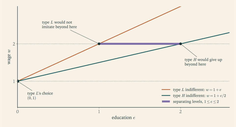
Figure 8.1 shows the two conditions geometrically. Each type’s indifference curves in the \((e,w)\) plane are straight lines with slope \(1/\theta\) : the less able type must be paid \(1\) per unit of education to stay indifferent and the able type only \(1/2\) . Through the point \((0,1)\) , the fate of anyone taken for type \(L\) , the two lines fan apart, and they reach the wage \(2\) at \(e=1\) and \(e=2\) . Between those points lies every \(e^\star\) that type \(H\) will accept and type \(L\) will not copy. If education cost the same for both types the two lines would coincide, the interval would shrink to a point, and no signal could separate them. A signal works only if it is cheaper for the type that wants to be recognized.
There is a continuum of separating equilibria and a continuum of pooling ones. In all the separating ones education is pure waste from a social point of view: it produces nothing, and its only function is to redistribute wages toward the able. If \(\lambda>1/2\) , even type \(H\) is worse off in the best separating equilibrium, with payoff \(1.5\) , than in the pooling equilibrium at \(e_p=0\) , with payoff \(1+\lambda\) .
8.5 Bluffing: a partially revealing equilibrium
In the previous two examples the sender’s types wanted different things to be believed. When one type wants to be mistaken for another and the receiver’s best response to full imitation would defeat it, equilibrium requires randomization, and the receiver’s belief lands strictly between the prior and certainty.
Example 8.4: A one-card poker game
Two players each put \(1\) in the pot. The sender is dealt a card, High or Low with probability \(1/2\) each, and looks at it. She can Fold, losing her stake, or Bet, adding \(1\) to the pot. If she bets, the receiver can Fold, losing his stake, or Call, adding \(1\) ; after a call the card is shown and High wins the pot for the sender while Low wins it for the receiver. The sender’s net payoffs are: \(-1\) if she folds; \(+1\) if she bets and the receiver folds; \(+2\) if she bets with High and is called; \(-2\) if she bets with Low and is called. The receiver’s payoffs are the negatives.
With High, betting is strictly better than folding whatever the receiver does. Could there be an equilibrium in which Low never bets? Then a bet would reveal High, the receiver would fold to every bet, and Low would gain by betting, getting \(+1\) instead of \(-1\) . Could Low always bet? Then a bet would reveal nothing, the receiver’s belief in High would be \(1/2\) , calling would yield \(\tfrac12(-2)+\tfrac12(2)=0>-1\) , the receiver would always call, and Low would lose \(2\) instead of \(1\) by betting. So Low must bluff with some probability \(\beta\in(0,1)\) , and for that she must be indifferent. For the receiver to keep her indifferent he must call with a probability \(\gamma\in(0,1)\) , so he must be indifferent as well.
The receiver’s belief. By Bayes’ rule, after a bet
The receiver is indifferent. Calling yields \(\mu\cdot(-2)+(1-\mu)\cdot 2=2-4\mu\) and folding yields \(-1\) . Equality requires \(\mu=3/4\) , hence \(1+\beta=4/3\) and \(\beta=1/3\) .
Low is indifferent. Betting yields \((1-\gamma)\cdot 1+\gamma\cdot(-2)=1-3\gamma\) and folding yields \(-1\) . Equality requires \(\gamma=2/3\) .
The perfect Bayesian equilibrium is: High always bets; Low bets with probability \(1/3\) ; the receiver calls a bet with probability \(2/3\) , with belief \(\mu(\text{High}\mid\text{Bet})=3/4\) . High’s expected payoff is \(\tfrac13\cdot 1+\tfrac23\cdot 2=\tfrac53\) , Low’s is \(-1\) , and the sender’s expected payoff before the deal is \(\tfrac12\cdot\tfrac53+\tfrac12\cdot(-1)=\tfrac13\) .
A bet moves the receiver’s belief from \(1/2\) to \(3/4\) : it is informative, though not conclusive. Bluffing is not a psychological trick here. Low bluffs just often enough that the receiver cannot profit by always folding, and the receiver calls just often enough that bluffing does not pay; and it is the bluffs that make the receiver willing to call the bets that High makes, which is where the sender’s profit comes from. The game is zero-sum, and an exercise confirms that \(1/3\) is its value in the sense of Chapter 4.
8.6 Which beliefs off the path are reasonable?
Definition 8.2 lets the receiver believe anything after an unexpected message. That freedom is what produced so many equilibria in Examples 8.2 and 8.3, and some of the beliefs involved are hard to defend. The best-known restriction asks the receiver to consider which types could conceivably have gained from the unexpected message.
Definition 8.4 (intuitive criterion). Fix a perfect Bayesian equilibrium of a signaling game, and let \(u^\star(\theta)\) be type \(\theta\) ’s equilibrium payoff. For a message \(m\) that no type sends, say that \(m\) is equilibrium dominated for type \(\theta\) if \(u^\star(\theta)\) is strictly greater than \(u_S(\theta,m,a)\) for every action \(a\) that is a best response of the receiver to \(m\) under some belief. The equilibrium fails the intuitive criterion if there is an unsent message \(m\) with two properties: \(m\) is not equilibrium dominated for at least one type; and some type \(\theta'\) would strictly gain by sending \(m\) , compared with \(u^\star(\theta')\) , against every best response of the receiver to \(m\) under beliefs that assign probability zero to all types for which \(m\) is equilibrium dominated. If \(m\) is equilibrium dominated for every type, no such beliefs exist and the criterion places no restriction at \(m\) .
The idea is a speech the deviating type could make: “I am sending \(m\) . You can see that the other type could not gain by this whatever you concluded, so you should conclude that it is I; and if you do, I gain.”
Example 8.5: Pruning the equilibria of the two signaling examples
The pooling equilibrium of Example 8.2. Both types get \(2\) . Consider the unsent message \(D\) . For type \(L\) , the best that could follow \(D\) is the skilled job, worth \(4-3=1<2\) . So \(D\) is equilibrium dominated for type \(L\) . For type \(H\) the skilled job after \(D\) is worth \(3>2\) , so \(D\) is not equilibrium dominated for her. Beliefs that give zero probability to type \(L\) after \(D\) put probability \(1\) on \(H\) ; the employer’s best response is then \(S\) ; and type \(H\) gets \(3>2\) . The pooling equilibrium fails the criterion. The separating equilibrium has no unsent messages and passes trivially.
Spence’s model. Take a separating equilibrium with \(e^\star>1\) and consider an education level \(e'\) with \(1<e'<e^\star\) . For type \(L\) , even the highest wage \(2\) after \(e'\) gives \(2-e'<1\) , her equilibrium payoff; so \(e'\) is equilibrium dominated for her. Employers who rule her out pay the wage \(2\) after \(e'\) , and type \(H\) gets \(2-e'/2>2-e^\star/2\) . Type \(H\) is not ruled out, since that same inequality says \(e'\) is not equilibrium dominated for her. So every separating equilibrium with \(e^\star>1\) fails. The equilibrium with \(e^\star=1\) passes. An unsent level \(e'>1\) is equilibrium dominated for both types, because even the wage \(2\) gives type \(L\) less than \(1\) and type \(H\) less than \(1.5\) , so the criterion places no restriction there. An unsent level \(e'<1\) is equilibrium dominated for neither type, so every belief is allowed, including the belief that the worker is of type \(L\) ; the wage \(1\) is then a best response, and against it neither type gains.
Take a pooling equilibrium at \(e_p\) , with payoffs \(1+\lambda-e_p\) and \(1+\lambda-e_p/2\) . An education level \(e'\) is equilibrium dominated for type \(L\) if \(2-e'<1+\lambda-e_p\) , that is, if \(e'>e_p+1-\lambda\) . Type \(H\) gains from \(e'\) at the wage \(2\) if \(2-e'/2>1+\lambda-e_p/2\) , that is, if \(e'<e_p+2(1-\lambda)\) . Since \(\lambda<1\) there are levels \(e'\) satisfying both, and for those the criterion’s test is met. Every pooling equilibrium fails.
Of the two continua of equilibria in Example 8.3, exactly one survives: separation with the least education that deters imitation, \(e^\star=1\) . The criterion delivers a sharp prediction where Definition 8.2 delivered almost none. It is not beyond dispute, however. When \(\lambda\) is close to \(1\) nearly everyone is able, and the surviving equilibrium has nearly everyone paying for wasteful education to distinguish themselves from a handful, although all would be better off pooling at zero. Refinements of equilibrium remain a matter of judgement about what unexpected behaviour means.
The equilibrium concepts of this book are now all on the table, and they are nested. In a signaling game, the strategies of every perfect Bayesian equilibrium form a Bayes–Nash equilibrium of the associated Bayesian game in which the receiver’s strategy is a plan \(a:M\to A\) : condition (S) is the sender’s interim optimality, and conditions (R) and (B) together say that the receiver’s plan is optimal against the sender’s strategy at every message that occurs. The converse fails, because a Bayes–Nash equilibrium lets the receiver plan anything at messages that do not occur. Likewise subgame-perfect equilibria are Nash equilibria that remain equilibria in every subgame, and backward induction is subgame perfection in trees with perfect information. Each refinement was introduced to remove equilibria that depend on behaviour which would not be rational if it were called upon.
Exercises
-
In Example 8.1 change the payoffs after \((R,r)\) from \((0,1)\) to \((0,3)\) . For which beliefs \(\mu\) , the probability of the node after \(L\) , is \(r\) sequentially rational? Find all perfect Bayesian equilibria in pure strategies, giving the beliefs that support each.
Solution
Let \(\mu\) be the probability player 2 assigns to the node after \(L\) . Now \(l\) yields \(\mu+2(1-\mu)=2-\mu\) and \(r\) yields \(0\cdot\mu+3(1-\mu)=3-3\mu\) . So \(r\) is sequentially rational exactly when \(3-3\mu\ge 2-\mu\) , that is, when \(\mu\le 1/2\) ; and \(l\) is sequentially rational exactly when \(\mu\ge 1/2\) .
Equilibria with \(L\) . If player 1 chooses \(L\) , the information set is reached and Bayes’ rule gives \(\mu=1\) , so player 2 must choose \(l\) . Against \(l\) , player 1 gets \(2\) from \(L\) , \(1\) from Out, and \(0\) from \(R\) , so \(L\) is optimal. The assessment (\(L\) , \(l\) , \(\mu=1\) ) is a perfect Bayesian equilibrium.
Equilibria with \(R\) . Player 1 gets \(0\) from \(R\) whatever player 2 does and \(1\) from Out, so \(R\) is never optimal.
Equilibria with Out. The information set is not reached and the belief is free. If player 2 plans \(l\) , player 1 prefers \(L\) (getting \(2\) ) to Out, so Out is not optimal. If player 2 plans \(r\) , player 1 gets \(0\) from \(L\) or \(R\) and \(1\) from Out, so Out is optimal; and \(r\) is sequentially rational provided \(\mu\le 1/2\) . So (Out, \(r\) , any \(\mu\le 1/2\) ) is a perfect Bayesian equilibrium.
Unlike in Example 8.1, the threat \(r\) can now be rationalized: player 2 must believe that if she is called upon to move, it is at least as likely to be after \(R\) as after \(L\) . That belief concerns an event of probability zero, and Definition 8.2 does not exclude it, although \(R\) is a move that could never benefit player 1.
-
A sender is of type \(H\) with prior probability \(0.3\) and otherwise of type \(L\) . Type \(H\) sends the message \(m_1\) with probability \(0.8\) and type \(L\) sends it with probability \(0.4\) ; otherwise each sends \(m_2\) . Compute the receiver’s posterior probability of \(H\) after each message, and check that the two posteriors average to the prior when weighted by the probabilities of the messages.
Answer
\(m_1\) has probability \(0.3\cdot 0.8+0.7\cdot 0.4=0.52\) , and the posterior of \(H\) after it is \(0.24/0.52=6/13\) . \(m_2\) has probability \(0.48\) , and the posterior is \(0.06/0.48=1/8\) . Check: \(0.52\cdot\tfrac{6}{13}+0.48\cdot\tfrac18=0.24+0.06=0.3\) .
-
In Example 8.2 let the prior probability of type \(H\) be \(0.8\) . Find all perfect Bayesian equilibria in pure strategies, treating each of the sender’s four strategies in turn and stating the off-path beliefs where they matter.
Solution
The employer chooses \(S\) exactly when the probability of \(H\) is at least \(3/4\) , and the prior \(0.8\) now exceeds that.
\(H\) sends \(D\) , \(L\) sends \(N\) . Beliefs are \(1\) after \(D\) and \(0\) after \(N\) , so the employer plays \(S\) after \(D\) and \(U\) after \(N\) . Type \(H\) gets \(3\) against \(2\) from \(N\) ; type \(L\) gets \(2\) against \(1\) from \(D\) . An equilibrium, exactly as with the prior \(1/2\) : the separating equilibrium does not depend on the prior.
\(H\) sends \(N\) , \(L\) sends \(D\) . Type \(L\) gets \(2-3=-1\) and would get \(4\) from \(N\) . Not an equilibrium.
Both send \(N\) . The belief after \(N\) is \(0.8\) , so the employer plays \(S\) and both types get \(4\) , the highest payoff in the game. No response to \(D\) could make a deviation worthwhile, since \(D\) costs something and the wage cannot exceed \(4\) . So any response to \(D\) that is optimal for some belief will do: \(S\) with a belief of at least \(3/4\) on \(H\) , or \(U\) with a belief of at most \(3/4\) . That gives two equilibria which differ only off the path.
Both send \(D\) . The belief after \(D\) is \(0.8\) , the employer plays \(S\) , and the types get \(3\) and \(1\) . Type \(L\) would get at least \(2\) from \(N\) . Not an equilibrium.
So there are three perfect Bayesian equilibria in pure strategies: the separating one, and pooling on \(N\) with the skilled job, in two versions. With an optimistic prior the employer hires everyone into the skilled job without evidence, and the signal is not needed; the separating equilibrium still exists, but in it type \(H\) pays for a degree and ends with \(3\) instead of \(4\) .
-
Prove from condition (B) that in a separating equilibrium of a signaling game every message that is sent leads to a posterior concentrated on one type, and that in a pooling equilibrium the posterior after the common message equals the prior.
Hint
In a separating equilibrium the set \(\{\theta':m^\star(\theta')=m\}\) has exactly one element for each message that is sent; put that into (B). In a pooling equilibrium the set is all of \(\Theta\) , and the denominator is \(\sum_{\theta'}p(\theta')=1\) .
-
A student describes the pooling equilibrium of Example 8.2 as: “Both types choose \(N\) ; the employer chooses \(U\) ; since \(D\) is never chosen we need not say what happens after it.” Then, pressed, adds: “After \(D\) the belief must be \(1/2\) by Bayes’ rule.” Explain both errors, and state the full set of off-path beliefs and responses that support the equilibrium.
Hint
An equilibrium of a signaling game specifies the receiver’s action after every message. Without the response to \(D\) one cannot check that neither type wants to send it. And Bayes’ rule does not apply after a message of probability zero. The equilibrium needs the response \(U\) after \(D\) , supported by any belief \(\mu(H\mid D)\le 3/4\) ; the belief \(1/2\) happens to be among them, but it is chosen, not derived.
-
In Spence’s model let \(\theta_L=1\) and \(\theta_H=3\) , with cost \(e/\theta\) and wage equal to expected productivity. Find the set of education levels \(e^\star\) for which a separating equilibrium exists, and the level selected by the intuitive criterion.
Answer
Type \(L\) does not imitate when \(1\ge 3-e^\star\) , that is, \(e^\star\ge 2\) . Type \(H\) prefers separating when \(3-e^\star/3\ge 1\) , that is, \(e^\star\le 6\) . Separating equilibria exist for \(e^\star\in[2,6]\) , and the intuitive criterion selects \(e^\star=2\) .
-
In Example 8.3, compare each type’s payoff in the separating equilibrium with \(e^\star=1\) and in the pooling equilibrium with \(e_p=0\) . For which \(\lambda\) are both types better off pooling?
Answer
Separating with \(e^\star=1\) : type \(L\) gets \(1\) and type \(H\) gets \(1.5\) . Pooling at \(e_p=0\) : both get \(1+\lambda\) . Type \(L\) always prefers pooling; type \(H\) prefers it when \(1+\lambda>1.5\) . Both are better off pooling when \(\lambda>1/2\) .
-
In the poker game of Example 8.4 let the bet be \(2\) instead of \(1\) , so that a called bet wins or loses \(3\) , with the stakes of \(1\) unchanged. Find the perfect Bayesian equilibrium and the sender’s expected payoff, and compare the frequency of bluffing and of calling with those of the example.
Solution
With High, betting dominates folding as before. The arguments of Example 8.4 against “Low never bets” and “Low always bets” still apply (if Low always bets, calling yields \(0>-1\) ), so Low bluffs with a probability \(\beta\in(0,1)\) and the receiver calls with a probability \(\gamma\in(0,1)\) .
Low indifferent. Betting yields \((1-\gamma)\cdot 1+\gamma\cdot(-3)=1-4\gamma\) and folding yields \(-1\) , so \(\gamma=1/2\) .
Receiver indifferent. With belief \(\mu\) in High after a bet, calling yields \(\mu(-3)+(1-\mu)\cdot 3=3-6\mu\) and folding yields \(-1\) , so \(\mu=2/3\) . By Bayes’ rule \(\mu=1/(1+\beta)\) , so \(\beta=1/2\) .
The equilibrium: High bets; Low bets with probability \(1/2\) ; the receiver calls with probability \(1/2\) and believes High with probability \(2/3\) after a bet. High’s payoff is \(\tfrac12\cdot 1+\tfrac12\cdot 3=2\) , Low’s is \(-1\) , and the sender’s expected payoff is \(1/2\) .
Compared with the example, a larger bet is bluffed more often (\(1/2\) against \(1/3\) ) and called less often (\(1/2\) against \(2/3\) ). A bigger bet risks more for the caller relative to the pot, so the receiver needs a larger share of bluffs among the bets to be willing to call; and the bluffer risks more, so she needs to be called less often. The sender’s advantage rises from \(1/3\) to \(1/2\) .
-
A sender’s type \(\theta\) is \(0\) or \(1\) with equal probability. The sender sends a costless message, “zero” or “one”; the receiver then chooses a real number \(a\) . The receiver’s payoff is \(-(a-\theta)^2\) and the sender’s is \(-(a-\theta-b)^2\) , where \(b>0\) measures the sender’s bias toward higher actions. Show that a separating equilibrium, in which each type reports truthfully, exists if and only if \(b\le 1/2\) , and that a pooling equilibrium exists for every \(b\) .
Solution
In any equilibrium the receiver’s action after a message is the mean of his posterior, since \(a\) minimizes the expected value of \((a-\theta)^2\) .
Separating. If type \(0\) says “zero” and type \(1\) says “one”, the receiver responds with \(a=0\) and \(a=1\) . Type \(0\) gets \(-(0-0-b)^2=-b^2\) from the truth and \(-(1-b)^2\) from lying. She tells the truth when \(b^2\le(1-b)^2\) , that is, when \(b\le 1/2\) . Type \(1\) gets \(-b^2\) from the truth and \(-(0-1-b)^2=-(1+b)^2\) from lying, so she always tells the truth: a sender biased upward never wants to understate. Both messages are sent, so there are no off-path beliefs to specify. The separating equilibrium exists if and only if \(b\le 1/2\) .
Pooling. Let both types say “zero”, and let the receiver hold the prior belief after either message, responding with \(a=1/2\) to both. After “zero” this belief is forced by condition (B); after “one” it is a permitted off-path belief. Since the action does not depend on the message, neither type can gain by changing the message. This holds for every \(b\) .
Talk is free here, so it can be believed only if the sender has no incentive to lie. When the bias is small the interests are close enough for the truth to be credible; when \(b>1/2\) the low type would claim to be high, and no message can be trusted.
-
In Example 8.2 let the degree cost type \(L\) only \(1.5\) , with the prior probability of \(H\) equal to \(1/2\) . Show that there is no separating equilibrium. Then find an equilibrium in which type \(H\) chooses \(D\) , type \(L\) randomizes between \(D\) and \(N\) , and the employer randomizes after \(D\) .
Solution
No separating equilibrium. If \(H\) sends \(D\) and \(L\) sends \(N\) , the employer plays \(S\) after \(D\) and \(U\) after \(N\) . Type \(L\) gets \(2\) from \(N\) and \(4-1.5=2.5\) from \(D\) , so she imitates. The reverse separation also fails: there type \(L\) sends \(D\) , is assigned to \(U\) , and gets \(2-1.5=0.5\) , less than the \(4\) she would get from \(N\) .
A partially separating equilibrium. Let \(H\) send \(D\) , let \(L\) send \(D\) with probability \(\beta\) , and let the employer choose \(S\) after \(D\) with probability \(s\) .
After \(N\) , only type \(L\) can have moved, so the belief in \(H\) is \(0\) and the employer chooses \(U\) .
After \(D\) , Bayes’ rule gives \(\mu(H\mid D)=\tfrac12/(\tfrac12+\tfrac12\beta)=1/(1+\beta)\) . The employer is willing to randomize only if indifferent, which requires \(\mu(H\mid D)=3/4\) , hence \(\beta=1/3\) .
Type \(L\) must be indifferent between her two messages. \(N\) gives \(2\) . \(D\) gives the expected wage \(4s+2(1-s)=2+2s\) minus \(1.5\) . Equality requires \(2+2s-1.5=2\) , so \(s=3/4\) .
Type \(H\) must prefer \(D\) : it gives \(2+2\cdot\tfrac34-1=2.5>2\) . So the equilibrium is: \(H\) chooses \(D\) ; \(L\) chooses \(D\) with probability \(1/3\) ; the employer chooses \(S\) with probability \(3/4\) after \(D\) , holding the belief \(3/4\) , and \(U\) after \(N\) . A degree raises the employer’s belief from \(1/2\) to \(3/4\) without proving ability, because the cheap degree is sometimes obtained by type \(L\) .
-
In Example 8.2 with the prior probability of type \(H\) equal to \(0.8\) , consider the pooling equilibrium on \(N\) in which the employer chooses \(S\) after \(N\) . Does it pass the intuitive criterion? Justify the answer by examining the message \(D\) for each type.
Answer
It passes. Both types get \(4\) in equilibrium. After \(D\) the best possible payoff is \(4-1=3\) for type \(H\) and \(4-3=1\) for type \(L\) ; both are below \(4\) , so \(D\) is equilibrium dominated for both types. By the proviso in Definition 8.4 the criterion then places no restriction at \(D\) , the only unsent message, and the equilibrium passes.
-
A sender is a Friend with probability \(p\) and an Enemy otherwise. The sender may offer a Gift or not. If no gift is offered both get \(0\) . If a gift is offered the receiver accepts or rejects. An accepted gift gives the sender \(1\) and gives the receiver \(1\) if the sender is a Friend and \(-1\) if an Enemy. A rejected gift gives the sender \(-1\) and the receiver \(0\) . Find all pure perfect Bayesian equilibria as a function of \(p\) .
Solution
The receiver accepts a gift when his belief \(\mu\) that the sender is a Friend satisfies \(\mu-(1-\mu)\ge 0\) , that is, \(\mu\ge 1/2\) . Both types of sender have the same payoffs: \(1\) from an accepted gift, \(-1\) from a rejected one, \(0\) from no gift.
Separating. If only the Friend offers, the receiver accepts, and then the Enemy gains by offering too (\(1>0\) ). If only the Enemy offers, the receiver rejects and the Enemy gets \(-1<0\) . No separating equilibrium exists; the Enemy can costlessly imitate.
Pooling on Gift. The belief after a gift is the prior \(p\) . If \(p\ge 1/2\) the receiver accepts, both types get \(1\) , and neither prefers \(0\) . This is an equilibrium exactly when \(p\ge 1/2\) . There is no off-path decision for the receiver.
Pooling on no gift. A gift is off the path, so the belief after it is free. If the receiver would reject, a deviator gets \(-1<0\) ; rejection is optimal for beliefs \(\mu\le 1/2\) . If the receiver would accept, both types deviate. So this is an equilibrium for every \(p\) , supported by a belief of at most \(1/2\) after an unexpected gift.
For \(p<1/2\) the only pure equilibrium has no gifts. For \(p\ge 1/2\) there are two: gifts given and accepted, and no gifts. In the second, a Friend refrains from a gift that would have been welcome, because an unexpected gift would be met with suspicion. Since both types have identical payoffs, no message is equilibrium dominated for one type and not the other, and the intuitive criterion cannot remove it.
-
Prove that the strategies of a pure perfect Bayesian equilibrium of a signaling game form a Bayes–Nash equilibrium of the game in which the sender’s strategies are functions \(\Theta\to M\) and the receiver’s are functions \(M\to A\) . Then give an example from this chapter of a Nash equilibrium that is not part of any perfect Bayesian equilibrium.
Hint
Condition (S) is the sender’s interim optimality for each type against the receiver’s plan. For the receiver, write his ex ante payoff as a sum over messages; the terms for messages that are sent are maximized by (R) with the beliefs of (B), and the terms for unsent messages have weight zero. For the example, look at Example 8.1, where (Out, \(r\) ) is a Nash equilibrium that no belief supports.
-
Show that in a finite extensive game with perfect information, the strategy profiles of perfect Bayesian equilibria are exactly the subgame-perfect equilibria of Chapter 6, and say what the beliefs are.
Hint
Every information set is a single node, so the only possible belief puts probability one on it. Sequential rationality at every node is then the condition used in the proof of Proposition 6.3.
-
Write the strategic form of the poker game of Example 8.4, with the sender’s four pure strategies (an action for each card) as rows and the receiver’s two as columns, each cell holding the sender’s expected payoff. Solve it as a matrix game by the methods of Chapter 4, with a certificate, and compare the optimal strategies with the equilibrium of the example.
Solution
A sender strategy is a pair (action with High, action with Low). Against Call, betting wins \(2\) with High and loses \(2\) with Low; against Fold, betting wins \(1\) ; folding loses \(1\) . Averaging over the two cards:
\[ \begin{array}{c|cc} & \text{Call} & \text{Fold}\\ \hline \text{(Bet, Bet)} & 0 & 1\\ \text{(Bet, Fold)} & \tfrac12 & 0\\ \text{(Fold, Bet)} & -\tfrac32 & 0\\ \text{(Fold, Fold)} & -1 & -1 \end{array} \]For instance (Bet, Fold) against Call gives \(\tfrac12\cdot 2+\tfrac12\cdot(-1)=\tfrac12\) . The last two rows are dominated by the first two. In the remaining \(2\times 2\) game let the sender play (Bet, Bet) with probability \(x\) : against Call she gets \(\tfrac12(1-x)\) and against Fold she gets \(x\) ; these are equal at \(x=\tfrac13\) , where both are \(\tfrac13\) . Let the receiver call with probability \(y\) : the first row gets \(1-y\) and the second \(\tfrac12y\) , equal at \(y=\tfrac23\) , where both are \(\tfrac13\) .
Certificate: the sender’s mixture \((\tfrac13,\tfrac23,0,0)\) earns \(\tfrac13\) against each column, and against the receiver’s mixture \((\tfrac23,\tfrac13)\) the four rows earn \(\tfrac13,\tfrac13,-1,-1\) . The value is \(1/3\) .
The mixture over plans corresponds exactly to the equilibrium of Example 8.4: High bets in both plans used, and Low bets under the plan (Bet, Bet), which has probability \(\tfrac13\) . The receiver calls with probability \(\tfrac23\) . In a zero-sum game the perfect Bayesian equilibrium and the minimax solution describe the same behaviour.
-
A seller’s product is Good or Bad. The buyer pays \(8\) if he believes it Good and \(4\) if he believes it Bad. The seller can attach a warranty, which costs a Good seller \(1\) in expected repairs and a Bad seller \(5\) . Show that there is a separating equilibrium in which only the Good seller offers the warranty, and say how the conclusion changes if the warranty costs the Bad seller \(3\) .
Answer
With the warranty read as Good and its absence as Bad: a Good seller gets \(8-1=7\) with it and \(4\) without; a Bad seller gets \(4\) without and \(8-5=3\) with. Neither deviates, so the equilibrium is separating. If the warranty costs the Bad seller \(3\) , he gets \(8-3=5>4\) by imitating, and separation breaks down.
-
A student says of Example 8.4: “With Low the sender should never bet: if called she loses \(2\) instead of \(1\) .” Find the receiver’s best response to a sender who never bluffs, then the sender’s best response to that, and explain why never bluffing cannot be part of an equilibrium.
Hint
If Low never bets, a bet proves High, and the receiver’s best response is to fold to every bet. Against a receiver who always folds, a bet with Low wins \(1\) instead of losing \(1\) . So “never bluff” is not a best response to the receiver’s best response to it.
-
In the Cournot game with private cost of Example 7.2, suppose firm 2 can make a costless public announcement, “low” or “high”, before quantities are chosen, and that firm 1 believes the announcement. Using the complete-information quantities from Chapter 7, compute what the high-cost type would earn by announcing “low”, and conclude that there is no equilibrium in which announcements are truthful and believed.
Solution
If firm 1 believes the announcement “low”, it believes the cost is \(0\) and produces the complete-information quantity \(q_1=10/3\) . A high-cost firm 2 that has announced “low” then best-responds to \(10/3\) with its true cost: \(q_2=(14-4-\tfrac{10}{3})/2=\tfrac{10}{3}\) , and earns \(q_2^2=100/9\approx 11.11\) . If it tells the truth, firm 1 produces \(14/3\) and firm 2 earns \(64/9\approx 7.11\) .
So the high-cost type gains by claiming to be low-cost, and an announcement that is always believed will not always be true. There is no equilibrium with truthful, believed announcements. Both types want firm 1 to think the cost is low, because that makes firm 1 cut back; when all types want to induce the same belief, a costless message cannot distinguish them, and firm 1 should ignore the announcement. For the low-cost type to be recognized it would need a signal that the high-cost type finds too expensive to copy, as in Example 8.2.