Arno and Bea, the café owners of Chapter 1, do not set prices once. They set them every Monday, each knowing what the other charged in all previous weeks, with no end in sight. Arno puts a proposal to Bea: “Let us both charge High. If either of us ever charges Low, the understanding is over and we both charge Low from then on.” In a single week Low is dominant and the proposal would be empty talk. Over many weeks it sounds persuasive: a price cut earns \(8\) instead of \(6\) once and costs the difference between \(6\) and \(3\) every week afterwards.
Two questions must be answered before the proposal can be called an equilibrium. First, is it really in each owner’s interest to keep charging High, week after week? That depends on how much the future matters to them. Second, is the punishment believable? If Bea cuts her price, would Arno carry out the reversion to Low for ever, or would he prefer to forgive her? The entry game of Chapter 5 taught us to ask this of every threat. But the weekly game is not a tree with perfect information, since each week’s prices are chosen simultaneously, and it has no last node from which to work backward. This chapter builds the concept that asks the credibility question in such games, proves a tool that makes the question answerable, and uses it to find out which outcomes of a repeated relationship can be sustained without any contract.
6.1 Subgames
Backward induction solved a tree by solving its parts. The parts were subtrees, and they made sense as games in their own right because everyone knew when play had entered one. With information sets that need not be so.
Definition 6.1 (subgame). Let \(\Gamma\) be an extensive game, possibly with imperfect information. A subgame of \(\Gamma\) consists of a decision node \(x\) and all the nodes that follow it, provided that (i) \(x\) is the only node in its information set, and (ii) every information set that contains a node following \(x\) contains only nodes following \(x\) . The whole game \(\Gamma\) is a subgame of itself; the others are proper subgames.
The two conditions say that when play reaches \(x\) this is common knowledge among the players, and that it remains so afterwards. A subgame is therefore a game: it has a root, players, information sets, and payoffs, and a strategy profile of \(\Gamma\) induces a strategy profile in it, by restriction.
Definition 6.2 (subgame-perfect equilibrium). A strategy profile of \(\Gamma\) is a subgame-perfect equilibrium if the profile it induces in every subgame of \(\Gamma\) is a Nash equilibrium of that subgame.
Since \(\Gamma\) is a subgame of itself, a subgame-perfect equilibrium is a Nash equilibrium; the definition adds the requirement that the strategies remain an equilibrium after every history that begins a subgame, whether or not that history occurs. A plan that would not be followed in some subgame, like Fight in the entry game, is thereby excluded.
Proposition 6.3 (perfect information). In a finite extensive game with perfect information, the subgame-perfect equilibria in pure strategies are exactly the backward-induction profiles.
Proof. With perfect information every decision node begins a subgame, the subtree at that node. A backward-induction profile induces a Nash equilibrium in every subtree by Theorem 5.3(a), so it is subgame perfect. Conversely, let \(s\) be subgame perfect and let \(x\) be any decision node, with mover \(i\) . In the subgame at \(x\) , player \(i\) could deviate by changing only the action at \(x\) ; since \(s\) induces a Nash equilibrium there, the action \(s\) prescribes at \(x\) gives \(i\) at least as much as any other action at \(x\) , given that \(s\) is followed afterwards. That is precisely the condition by which backward induction selects the action at \(x\) , so \(s\) can be produced by the procedure.
Theorem 6.4 (existence). Every finite extensive game with perfect recall has a subgame-perfect equilibrium, possibly in mixed strategies.
Proof. We argue by induction on the number of subgames, treating a mixed strategy as a behaviour strategy, an independent randomization at each information set. With perfect recall nothing is lost by this: every mixed strategy has a behaviour strategy that gives the same distribution over outcomes against all strategies of the others, a fact known as Kuhn’s theorem that we use without proof. So equilibria may be taken in behaviour strategies, and only deviations to behaviour strategies need to be considered; such strategies can be cut into a part inside a subgame and a part outside it, which is what the argument requires. If \(\Gamma\) has no proper subgame, any Nash equilibrium of \(\Gamma\) , which exists by Theorem 4.7 applied to the strategic form, is subgame perfect. Otherwise choose a proper subgame, beginning at \(x\) , that has no proper subgames of its own, and let \(\sigma^x\) be a Nash equilibrium of it, with payoff vector \(v(x)\) . Replace the subgame by a terminal node with payoffs \(v(x)\) . The resulting game still has perfect recall, since its information sets are information sets of \(\Gamma\) and no player has forgotten anything in \(\Gamma\) ; and it has fewer subgames, so it has a subgame-perfect equilibrium \(\sigma'\) . Let \(\sigma\) follow \(\sigma^x\) inside the subgame at \(x\) and \(\sigma'\) elsewhere. In any subgame containing \(x\) , a player’s deviation can change that player’s payoff after \(x\) only downward, because \(\sigma^x\) is an equilibrium of the subgame at \(x\) ; so the deviation earns no more than the same deviation outside \(x\) would earn in the reduced game, which is not profitable. Hence \(\sigma\) induces a Nash equilibrium in every subgame.
The proof is a recipe: solve the smallest subgames, replace them by their equilibrium payoffs, and continue toward the root. When a subgame has several equilibria the recipe branches, as the next example shows.
Example 6.1: Entry followed by a simultaneous contest
A rival chooses Out, which ends the game with payoffs \((0,4)\) to rival and incumbent, or In. After In the two firms choose simultaneously: the rival builds a Large or a Small store, and the incumbent chooses to Fight or to Share. The payoffs after In are
The game has one proper subgame, beginning after In; inside it the incumbent’s two nodes form one information set, so nothing smaller is a subgame.
Equilibria of the subgame. Marking best responses gives two pure equilibria, (Large, Share) with payoffs \((3,1)\) and (Small, Fight) with payoffs \((-1,3)\) . There is also a mixed one. The incumbent is indifferent when \(-p+3(1-p)=p+2(1-p)\) , where \(p\) is the probability of Large, so \(p=1/3\) ; the rival is indifferent when \(-3q+3(1-q)=-q+(1-q)\) , where \(q\) is the probability of Fight, so \(q=1/2\) . The mixed equilibrium gives the rival \(0\) and the incumbent \(5/3\) .
The first move. Replace the subgame by each equilibrium payoff in turn. If (Large, Share) will follow entry, the rival compares \(3\) with \(0\) and enters. If (Small, Fight) will follow, the rival compares \(-1\) with \(0\) and stays out. If the mixed equilibrium will follow, the rival gets \(0\) either way and any choice, including a random one, is optimal.
So the subgame-perfect equilibria are: In followed by (Large, Share); Out, with (Small, Fight) as the plan after entry; and any first move together with the mixed plan. Unlike in Chapter 5, fighting can now be part of a subgame-perfect equilibrium. The reason is that here Fight is a best response to something the rival might do after entering, namely Small, and Small is a best response to Fight. Subgame perfection removes plans that are not equilibria of the continuation; it does not choose among continuation equilibria.
6.2 Repetition
Definition 6.5 (repeated game). Let \(G\) be a game in strategic form with action sets \(A_i\) and payoff functions \(u_i\) , called the stage game. In the repeated game, \(G\) is played in periods \(t=0,1,2,\dots\) ; before each period all players observe the actions chosen in all earlier periods. A history of length \(t\) is a list \(h=(a^0,\dots,a^{t-1})\) of action profiles, and a strategy of player \(i\) assigns an action in \(A_i\) to every history of every length. In the \(T\) -period repeated game there are \(T\) periods and a player’s payoff is \(\sum_{t=0}^{T-1}\delta^tu_i(a^t)\) , where \(\delta\in(0,1]\) and \(\delta=1\) means that the stage payoffs are simply added. In the infinitely repeated game with discount factor \(\delta\in(0,1)\) the payoff is
Every history begins a subgame, because all past actions are observed, and the subgame after a history of the infinitely repeated game is a copy of the whole game. The stage game’s strategies are called actions here to keep them apart from strategies of the repeated game, which are far more numerous: a strategy is a rule for all contingencies.
The discount factor measures the weight of the future. It can represent patience, with \(\delta=1/(1+r)\) for an interest rate \(r\) per period; or the probability that the relationship continues for another period, the game ending for ever with probability \(1-\delta\) after each round; or both together. A constant payoff \(c\) per period is worth \(c+\delta c+\delta^2c+\dots=c/(1-\delta)\) . Multiplying \(U_i\) by \((1-\delta)\) gives the normalized payoff, which is expressed in the units of the stage game: the normalized payoff of receiving \(c\) every period is \(c\) .
6.3 The one-shot deviation principle
To check that a profile is subgame perfect one must show that, after every history, no player has any profitable deviation; and a deviation in a repeated game is an entire alternative strategy, which may differ from the original after infinitely many histories. That looks unmanageable. The following theorem cuts the task down to a finite check in every example of this chapter.
A one-shot deviation from a strategy \(s_i\) is a strategy that differs from \(s_i\) at exactly one history \(h\) , prescribing a different action there and agreeing with \(s_i\) everywhere else, in particular at all later histories.
Theorem 6.6 (one-shot deviation principle). Consider a finitely repeated game, or an infinitely repeated game with discount factor \(\delta<1\) whose stage payoffs are bounded. A profile \(s\) of pure strategies is a subgame-perfect equilibrium if and only if no player has a profitable one-shot deviation: for every player \(i\) and every history \(h\) , the strategy \(s_i\) does at least as well in the subgame after \(h\) as any strategy that differs from \(s_i\) only at \(h\) , given \(s_{-i}\) .
Proof. A one-shot deviation at \(h\) is in particular a deviation in the subgame after \(h\) , so the condition is necessary. For sufficiency, suppose no one-shot deviation is profitable and yet, after some history \(h\) , player \(i\) has a strategy \(s_i'\) that earns \(\varepsilon>0\) more than \(s_i\) in the subgame after \(h\) , against \(s_{-i}\) . Count periods from \(h\) .
Step 1: finitely many periods suffice. In the infinite case let \(M\) bound the absolute value of the stage payoffs. Whatever is done from period \(T\) on changes a player’s payoff by at most \(2M\delta^{T}/(1-\delta)\) , which is less than \(\varepsilon/2\) for \(T\) large. Let \(s_i''\) agree with \(s_i'\) in the first \(T\) periods after \(h\) and with \(s_i\) thereafter. Then \(s_i''\) earns more than \(s_i\) in the subgame after \(h\) . In the finite case take \(s_i''=s_i'\) and let \(T\) be the number of remaining periods.
Step 2: removing the last period of deviation never hurts. For \(k=0,1,\dots,T\) let \(s_i^{(k)}\) agree with \(s_i''\) in the first \(k\) periods after \(h\) and with \(s_i\) afterwards, so that \(s_i^{(T)}=s_i''\) and \(s_i^{(0)}=s_i\) . Compare \(s_i^{(k)}\) with \(s_i^{(k-1)}\) . They prescribe the same actions in the first \(k-1\) periods, so against \(s_{-i}\) they lead to the same history \(\hat h\) at the start of period \(k\) . At \(\hat h\) the first follows \(s_i''\) for one period and then \(s_i\) ; the second follows \(s_i\) throughout. So in the subgame after \(\hat h\) the first is a one-shot deviation from \(s_i\) , or coincides with it, and by hypothesis earns no more there. The payoffs before \(\hat h\) are the same. Hence \(s_i^{(k-1)}\) earns at least as much as \(s_i^{(k)}\) in the subgame after \(h\) .
Chaining these inequalities from \(k=T\) down to \(k=1\) shows that \(s_i=s_i^{(0)}\) earns at least as much as \(s_i''=s_i^{(T)}\) , contradicting Step 1.
The principle is the game-theoretic form of the principle of optimality in dynamic programming, treated in Dynamic Programming and Optimal Control: a plan is optimal if and only if it cannot be improved by changing a single decision. The proof used nothing about the stage game beyond bounded payoffs and the fact that every history begins a subgame. It therefore applies equally when each period’s game is itself a game with perfect information in which the players move in turn: a history is then any sequence of past moves, including moves already made in the current period, and a one-shot deviation changes the action at one decision node. Two cautions. The condition must hold at every history, including those that the profile itself never reaches; checking only the histories on the equilibrium path establishes a Nash equilibrium at most. And discounting is needed in Step 1: without it, gains pushed infinitely far into the future could not be ignored.
6.4 A known last period
Proposition 6.7 (unravelling). If the stage game \(G\) has a unique Nash equilibrium \(a^\star\) , then for every finite \(T\) the \(T\) -period repeated game has a unique subgame-perfect equilibrium: every player \(i\) plays \(a_i^\star\) after every history.
Proof. By induction on \(T\) . For \(T=1\) the claim is the hypothesis. Suppose it holds for \(T-1\) and consider a subgame-perfect equilibrium of the \(T\) -period game. After each first-period profile \(a^0\) the remaining game is a \((T-1)\) -period repeated game, so by the induction hypothesis the continuation is \(a^\star\) in every remaining period whatever \(a^0\) was. Each player’s total payoff is therefore \(u_i(a^0)\) plus a constant that does not depend on \(a^0\) . So the first-period actions must form a Nash equilibrium of \(G\) , and that is \(a^\star\) .
Example 6.2: Ten weeks of price competition
Suppose Arno and Bea know that the square will be closed for rebuilding after week 10. The stage game has the unique equilibrium (Low, Low), since Low is strictly dominant. By Proposition 6.7 the unique subgame-perfect equilibrium is Low by both in every week after every history, with \(3\) per week each.
The trigger proposal fails for a simple reason. In week 10 there is no future, so both charge Low whatever happened before. In week 9, then, the threat “or else Low in week 10” has no force, because Low in week 10 is coming anyway; so both charge Low in week 9. The same goes for week 8, and the argument unravels to week 1. Compare the sums: ten weeks of (High, High) would give each owner \(60\) , and the equilibrium gives \(30\) . A known end date destroys cooperation in this model however distant it is, a conclusion as uncomfortable as the centipede’s, and for the same reason.
Unravelling depends on the uniqueness of the stage equilibrium. If the stage game has two equilibria, the choice between them in the last period can depend on earlier behaviour, and that dependence is a credible reward and punishment.
Example 6.3: Two stage equilibria support cooperation for one period
Let the stage game be
Its pure Nash equilibria are \((D,D)\) with payoffs \((1,1)\) and \((G,G)\) with payoffs \((3,3)\) . The profile \((C,C)\) , with the highest payoffs, is not an equilibrium: each player would switch to \(D\) and get \(5\) .
Play the game twice, without discounting. Consider the profile: in the first period play \(C\) ; in the second period play \(G\) if the first-period outcome was \((C,C)\) and play \(D\) otherwise. By Theorem 6.6 it is enough to rule out one-shot deviations. In the second period, after any history, the prescribed actions form a Nash equilibrium of the stage game, \((G,G)\) or \((D,D)\) , and there is no future; no deviation gains. In the first period, conforming yields \(4+3=7\) . The best deviation is to \(D\) , which yields \(5\) now and then \((D,D)\) , for a total of \(5+1=6<7\) . So the profile is a subgame-perfect equilibrium, and the non-equilibrium outcome \((C,C)\) is played in the first period.
With a discount factor \(\delta\) applied to the second period the comparison is \(4+3\delta\ge 5+\delta\) , which holds exactly when \(\delta\ge\tfrac12\) .
6.5 No last period
In the infinitely repeated game there is no final period from which to unravel. Arno’s proposal is a strategy: charge High at the start and after every history in which nobody has ever charged Low; charge Low after every other history. It is called the grim trigger strategy.
Example 6.4: When is the grim trigger an equilibrium?
Let both owners use the grim trigger. The stage payoffs are \(6\) each at (High, High), \(3\) each at (Low, Low), \(8\) to an owner who charges Low against High, and \(1\) to the other. Histories are of two kinds, and by Theorem 6.6 we need to examine one deviation at each kind.
Histories with no Low so far. Conforming gives \(6\) in every period, worth \(6/(1-\delta)\) . A one-shot deviation to Low gives \(8\) today; from tomorrow both strategies prescribe Low for ever, worth \(3\) per period, so the deviation is worth \(8+3\delta/(1-\delta)\) . Conforming is at least as good when
Histories containing a Low. Both strategies prescribe Low for ever. Conforming gives \(3\) today. A one-shot deviation to High gives \(1\) today and changes nothing afterwards, since the history still contains a Low. It loses \(2\) .
So the grim-trigger profile is a subgame-perfect equilibrium if and only if \(\delta\ge 2/5\) . The answer to the first question of this chapter is that cooperation is in each owner’s interest when the future has enough weight: with an interest rate \(r\) per week, \(\delta=1/(1+r)\ge 2/5\) means \(r\le 150\%\) , and with a weekly probability \(\delta\) of the relationship continuing, it means that the relationship is expected to last. The answer to the second question is that the punishment is credible because it consists of playing the stage-game equilibrium for ever, which is itself a subgame-perfect equilibrium of the repeated game.
In a general prisoner’s dilemma with payoffs \(T>R>P>S\) (the temptation, the reward for mutual cooperation, the punishment for mutual defection, and the payoff of an exploited cooperator), the same computation gives the condition \(\delta\ge(T-R)/(T-P)\) : the one-period gain from cheating relative to the per-period loss in the punishment phase.
The grim trigger is not the only way to try to sustain cooperation, and other natural strategies fail a test that it passes.
Example 6.5: Tit-for-tat is not credible
Tit-for-tat charges High in the first week and thereafter charges whatever the other owner charged the week before. If both owners use it, they charge High for ever, as with the grim trigger. What tit-for-tat prescribes depends only on the previous week’s prices, so there are four kinds of history to examine. Take Arno’s point of view, and use the fact that a path alternating between payoffs \(x\) and \(y\) is worth \((x+\delta y)/(1-\delta^2)\) .
After (High, High), or at the start. Conforming is worth \(6/(1-\delta)=(6+6\delta)/(1-\delta^2)\) . A one-shot deviation to Low yields \(8\) ; next week Bea copies the Low while Arno, back on tit-for-tat, copies her High; and the two then alternate for ever, which is worth \((8+\delta)/(1-\delta^2)\) to Arno. Conforming is at least as good when \(6+6\delta\ge 8+\delta\) , that is, \(\delta\ge 2/5\) .
After Arno charged High and Bea charged Low. Tit-for-tat tells Arno to punish with Low while Bea, copying his High, returns to High; then they alternate, worth \((8+\delta)/(1-\delta^2)\) to Arno. A one-shot deviation is to forgive: charge High. Then both have just charged High and cooperation resumes, worth \((6+6\delta)/(1-\delta^2)\) . Conforming is at least as good when \(8+\delta\ge 6+6\delta\) , that is, \(\delta\le 2/5\) .
The two conditions are compatible only at the single value \(\delta=2/5\) . The remaining two kinds of history give the same pair of conditions. So for every \(\delta>2/5\) tit-for-tat fails to be subgame perfect, although, as one can check by comparing it with all of Arno’s alternatives along the path, it is a Nash equilibrium for all \(\delta\ge 2/5\) . The failure is off the path: after a single lapse, tit-for-tat demands an endless echo of alternating punishments, and a patient owner would rather forgive. The punishment is not believable, and by the logic of Chapter 5 a threat that would not be carried out should not deter. The grim trigger does not have this defect; its punishment is harsher, yet each owner is willing to carry it out because the other is doing the same.
Common mistake. Checking a repeated-game strategy only along the path it generates. Showing that neither player gains by deviating from High when both follow tit-for-tat proves that the profile is a Nash equilibrium. Subgame perfection requires the same check after every history, in particular after histories in which someone has already deviated, where the strategy prescribes the punishment. For each proposed profile, list the kinds of history the strategies distinguish (their “states”), and test a one-shot deviation in each state for each player. A second mistake is to apply trigger reasoning to a game with a known final period: Proposition 6.7 shows that when the stage equilibrium is unique no punishment is available at the end, and so none is available before it.
6.6 What repetition can sustain
The grim trigger shows that (High, High) can be sustained. What else can? It is useful to have upper and lower limits on what any equilibrium of the repeated game can give the players.
Definition 6.8 (feasible and individually rational payoffs). The set \(F\) of feasible payoff vectors of the stage game is the convex hull of the vectors \(u(a)=(u_1(a),\dots,u_n(a))\) over all action profiles \(a\) . Player \(i\) ’s minmax payoff is
where \(\alpha_{-i}\) ranges over the mixed action profiles of the other players. A payoff vector \(v\) is individually rational if \(v_i\ge\underline v_i\) for every \(i\) , and strictly so if every inequality is strict.
The minmax payoff is the lowest payoff to which the others can hold player \(i\) when \(i\) knows what they are doing and replies optimally. In the café game, if Bea charges Low the best Arno can get is \(3\) , and if she charges High he can get \(8\) ; so \(\underline v_i=3\) , attained when the opponent charges Low.
Proposition 6.9 (limits on equilibrium payoffs). In every Nash equilibrium of the infinitely repeated game, for every \(\delta\) , the vector of normalized payoffs is feasible and individually rational.
Proof. The normalized payoff vector is \(\sum_t(1-\delta)\delta^tu(a^t)\) , averaged over the randomness of play if strategies are mixed. The weights \((1-\delta)\delta^t\) are nonnegative and sum to \(1\) , so this is a convex combination of vectors \(u(a)\) and lies in \(F\) . For individual rationality, let player \(i\) deviate to the strategy that, after each history, plays a best response to the mixed action the others are about to play. In every period \(i\) ’s expected stage payoff is then at least \(\underline v_i\) , so the normalized payoff of the deviation is at least \(\underline v_i\) . An equilibrium payoff is at least that.
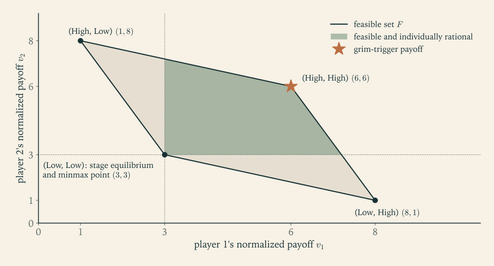
Figure 6.1 shows \(F\) for the café game: the quadrilateral with corners \((3,3)\) , \((1,8)\) , \((6,6)\) , and \((8,1)\) . The individually rational part is cut off by the lines \(v_1=3\) and \(v_2=3\) . Proposition 6.9 says that no equilibrium payoff lies outside the shaded region. The remarkable fact is that, for patient players, essentially everything inside it is an equilibrium payoff. We prove the simplest version.
Theorem 6.10 (Nash-reversion folk theorem). Let \(a^N\) be a Nash equilibrium in pure actions of the stage game, with payoffs \(e_i=u_i(a^N)\) , and let \(a\) be a pure action profile with \(u_i(a)>e_i\) for every player \(i\) . Suppose the stage payoffs are bounded and each maximum \(d_i=\max_{a_i'}u_i(a_i',a_{-i})\) , player \(i\) ’s best payoff from a unilateral deviation from \(a\) , is attained, and put
Then \(\delta_0<1\) , and the following profile, whose normalized payoffs are \(u(a)\) , is a subgame-perfect equilibrium of the infinitely repeated game if and only if \(\delta\ge\delta_0\) : play \(a\) at the start and after every history in which \(a\) was played in every period; after every other history play \(a^N\) .
Proof. Since \(u_i(a)>e_i\) and \(d_i\ge u_i(a)\) , each ratio lies in \([0,1)\) , so \(\delta_0<1\) . By Theorem 6.6 the profile is subgame perfect exactly when no one-shot deviation is profitable. After a history at which \(a^N\) is prescribed, it is prescribed for ever whatever anyone does now; a deviation changes only today’s payoff, and cannot raise it because \(a^N\) is a Nash equilibrium of the stage game. After a history at which \(a\) is prescribed, conforming is worth \(u_i(a)/(1-\delta)\) and the best one-shot deviation is worth \(d_i+\delta e_i/(1-\delta)\) . Conforming is at least as good exactly when \(u_i(a)\ge(1-\delta)d_i+\delta e_i\) , that is, when \(\delta(d_i-e_i)\ge d_i-u_i(a)\) . Since \(d_i-e_i>0\) , this holds for every player if and only if \(\delta\ge\delta_0\) ; for a player with \(d_i=u_i(a)\) it holds for every \(\delta\) .
For the cafés, \(a=\) (High, High), \(e_i=3\) , \(d_i=8\) , and \(\delta_0=(8-6)/(8-3)=2/5\) , as found in Example 6.4.
The full result goes much further. We state it without proof. Suppose there are two players, or that \(F\) has dimension \(n\) , and that the players can observe a public random signal at the start of each period. Then for every feasible and strictly individually rational payoff vector \(v\) there is a \(\delta_0<1\) such that for every \(\delta\in(\delta_0,1)\) the infinitely repeated game has a subgame-perfect equilibrium with normalized payoffs \(v\) . This is the folk theorem, in the form proved by Fudenberg and Maskin. The punishments it uses are harsher than Nash reversion, holding a deviator to the minmax payoff for a while, and they include rewards to the punishers for carrying them out, which is what makes them credible.
The folk theorem has two faces. It explains how cooperation can be sustained among self-interested parties with no contract and no outside enforcement, and it identifies what is needed: observable actions, an indefinite horizon, and enough patience. But it also says that the repeated game has an enormous number of equilibria, among them the endless repetition of the one-shot equilibrium, and the theory does not say which one will be played. In the repeated café game “cooperation is an equilibrium” is a theorem, and “the owners will cooperate” is not.
Example 6.6: Collusion in quantities
Let the Cournot duopolists of Example 2.3 meet in every period. With quantities unrestricted the stage payoffs are unbounded below, since a firm can lose any amount by flooding the market, and Theorems 6.6 and 6.10 assume bounded payoffs. So restrict each firm to quantities in \([0,14]\) . Nothing is lost: an output above \(12\) earns a negative profit whatever the rival does, so it is never part of a best response or a profitable deviation, and with the restriction every stage profit lies between \(-28\) and \(36\) . The same restriction is understood whenever a quantity game is repeated in the exercises. The stage equilibrium is \(4\) each with profit \(e_i=16\) . The joint-profit-maximizing profile is \(a=(3,3)\) with profit \(18\) each, and the best deviation from it is the reply \(4.5\) , with profit \(d_i=20.25\) . By Theorem 6.10, producing \(3\) each, with reversion to \(4\) each for ever after any deviation, is a subgame-perfect equilibrium exactly when
Less ambitious agreements need less patience. If the firms produce \(3.5\) each, each earns \(3.5\cdot 5=17.5\) ; the best reply to \(3.5\) is \(4.25\) , with profit \(4.25^2=18.0625\) ; and the threshold is \((18.0625-17.5)/(18.0625-16)=0.5625/2.0625=3/11\approx 0.273\) . Between full collusion and none there is a continuum of sustainable outcomes, each with its own critical discount factor.
Subgame perfection has now been pushed as far as it goes: it rules out a plan that is not an equilibrium of some subgame. Many games have few subgames. If a player does not know something that another player knows, about a past move or about the other player’s payoffs, information sets spread across the tree and there may be no proper subgame at all. The next two chapters deal with private information, first in static games and then in dynamic ones, where a new idea is needed to do the work that subgames do here.
Exercises
-
Player 1 chooses \(L\) or \(R\) . After \(L\) , players 2 and 3 choose simultaneously, each between two actions. After \(R\) , player 2 chooses between two actions, observed by player 3, who then chooses between two actions. Describe the information sets, and count the subgames of this game, including the whole game.
Answer
After \(L\) , player 2 has one node and player 3 has two nodes in a single information set. After \(R\) , player 2 has one node and player 3 has two nodes, each its own information set. The subgames are: the whole game; the game after \(L\) ; the game after \(R\) ; and the two one-player games at player 3’s nodes after \(R\) . That is \(5\) subgames. Player 3’s nodes after \(L\) do not begin subgames.
-
Player 1 chooses Out, ending the game with payoffs \((1.5,1.5)\) , or In, after which the two players play the seminar game of Chapter 2 simultaneously. Find all subgame-perfect equilibria, including any that use the mixed equilibrium of the seminar game.
Solution
The only proper subgame is the seminar game after In. From Chapter 3 it has three Nash equilibria: (Algebra, Algebra) with payoffs \((2,1)\) ; (Biology, Biology) with payoffs \((1,2)\) ; and the mixed equilibrium, in which player 1 chooses Algebra with probability \(2/3\) and player 2 with probability \(1/3\) , with payoffs \((2/3,2/3)\) .
Replace the subgame by each equilibrium payoff and let player 1 choose between that and the \(1.5\) from Out.
If (Algebra, Algebra) follows In, player 1 compares \(2\) with \(1.5\) and chooses In.
If (Biology, Biology) follows In, player 1 compares \(1\) with \(1.5\) and chooses Out.
If the mixed equilibrium follows In, player 1 compares \(2/3\) with \(1.5\) and chooses Out.
There are three subgame-perfect equilibria: (In, then Algebra; Algebra), with payoffs \((2,1)\) ; (Out, with the plan Biology; Biology), with payoffs \((1.5,1.5)\) ; and (Out, with both players planning the mixed strategies), with payoffs \((1.5,1.5)\) . In each, the plan after In is an equilibrium of the seminar game, as Definition 6.2 requires, and the first move is optimal given the plan.
-
Prove that every subgame-perfect equilibrium is a Nash equilibrium, and that in a game with no proper subgames the two concepts coincide. Then name a game from Chapter 5 that has a Nash equilibrium which is not subgame perfect.
Hint
The whole game is one of its own subgames, so Definition 6.2 includes the Nash condition for the whole game. If there are no proper subgames the definition contains nothing else. For the example, look at the first game of Chapter 5.
-
The café game is played twice, with payoffs added. Show that every subgame-perfect equilibrium has (Low, Low) in both periods after every history. Then show that the following profile is a Nash equilibrium but not subgame perfect: play Low in the first period; in the second period play High if the first-period outcome was (High, High) and Low otherwise.
Solution
Subgame-perfect equilibria. The stage game has the unique Nash equilibrium (Low, Low), because Low is strictly dominant. By Proposition 6.7 with \(T=2\) , the only subgame-perfect equilibrium plays Low after every history: in the second period every subgame is the stage game itself, so (Low, Low) is played after each first-period outcome; the first-period payoffs are then the stage payoffs plus the constant \(3\) , and Low is again dominant.
The proposed profile is a Nash equilibrium. If both follow it, the outcome is (Low, Low) twice and each owner gets \(3+3=6\) . Consider any deviation by owner 1. Owner 2 charges Low in the first period, so the first-period outcome is not (High, High) whatever owner 1 does, and owner 2 charges Low in the second period too. Against Low in both periods, owner 1 gets at most \(3\) per period, so at most \(3+3=6\) . No deviation gains, and by symmetry the same holds for owner 2.
It is not subgame perfect. In the subgame after the first-period outcome (High, High), the profile prescribes (High, High), which is not a Nash equilibrium of the stage game: either owner gains \(2\) by charging Low. The subgame is never reached, and a single owner cannot reach it alone, which is why the Nash test does not notice.
-
In the two-period game of Example 6.3, suppose the stage payoff at \((G,G)\) is \((2,2)\) instead of \((3,3)\) , and there is no discounting. Is the profile “play \(C\) , then \(G\) after \((C,C)\) and \(D\) otherwise” still a subgame-perfect equilibrium? Find the smallest payoff at \((G,G)\) for which it is.
Answer
With \((2,2)\) at \((G,G)\) , conforming yields \(4+2=6\) and the best deviation yields \(5+1=6\) . The deviation is not profitable, so the profile is still a subgame-perfect equilibrium, though no longer a strict one. In general the condition is \(4+g\ge 6\) , so \(g=2\) is the smallest payoff that works; and \((G,G)\) remains a stage equilibrium for any \(g\ge 0\) .
-
For the prisoner’s dilemma with payoffs \(T=5\) , \(R=3\) , \(P=1\) , \(S=0\) , find the values of \(\delta\) for which the grim-trigger profile is a subgame-perfect equilibrium, examining both kinds of history.
Answer
With no defection so far: \(3/(1-\delta)\ge 5+\delta/(1-\delta)\) , that is, \(3\ge 5-4\delta\) , so \(\delta\ge 1/2\) . After a defection: cooperating against a defector gives \(0<1\) today and changes nothing later, so there is no profitable deviation. The profile is subgame perfect exactly for \(\delta\ge 1/2=(T-R)/(T-P)\) .
-
In the repeated café game consider the strategy: charge High; if in any period anything other than the prescribed prices is observed, charge Low for \(k\) periods and then return to High, restarting the \(k\) periods of Low if anyone departs from Low during the punishment. Find the values of \(\delta\) for which this is a subgame-perfect equilibrium when \(k=1\) and when \(k=2\) , and say what happens to the threshold as \(k\to\infty\) .
Solution
The strategy distinguishes the cooperative state and \(k\) punishment states, according to how many periods of Low remain. By Theorem 6.6 it is enough to test one-shot deviations in each state.
In a punishment state the prescription is (Low, Low). Conforming gives \(3\) today and moves the punishment forward. Deviating to High gives \(1\) today and restarts the punishment, which postpones the return to \(6\) . The deviation is worse today and worse afterwards, for every \(\delta\) .
In the cooperative state conforming gives \(6\) in every period. A deviation to Low gives \(8\) today, then \(3\) for \(k\) periods, then \(6\) again from period \(k+1\) on. The two paths differ only in the first \(k+1\) periods, so conforming is at least as good when
\[ 6+6(\delta+\dots+\delta^k)\ \ge\ 8+3(\delta+\dots+\delta^k)\quad\Longleftrightarrow\quad 3(\delta+\delta^2+\dots+\delta^k)\ge 2 . \]For \(k=1\) this is \(3\delta\ge 2\) , that is, \(\delta\ge 2/3\) . For \(k=2\) it is \(3\delta^2+3\delta-2\ge 0\) , that is, \(\delta\ge(\sqrt{33}-3)/6\approx 0.457\) .
As \(k\to\infty\) the sum tends to \(\delta/(1-\delta)\) and the condition becomes \(3\delta\ge 2(1-\delta)\) , that is, \(\delta\ge 2/5\) , the grim-trigger threshold. Longer punishments deter with less patience, and the grim trigger is the limiting case. Shorter punishments need more patience but have the advantage that a single mistake does not end cooperation for ever.
-
In the repeated café game consider the strategy: charge High at the start; thereafter charge High if both owners charged the same price in the previous period and Low if they charged different prices. Identify the two kinds of history this strategy distinguishes, test a one-shot deviation at each, and find the values of \(\delta\) for which the profile is a subgame-perfect equilibrium.
Solution
The strategy’s prescription depends only on whether last period’s prices matched. Call the state match (prescription High; this includes the start) and mismatch (prescription Low). Both owners are always in the same state, since both observe the same prices.
State match. Conforming gives (High, High) for ever: \(6\) in every period. A one-shot deviation to Low gives \(8\) today and produces a mismatch; next period both charge Low, earning \(3\) , which is a match; from then on both charge High again. The paths differ in two periods only, so conforming is at least as good when \(6+6\delta\ge 8+3\delta\) , that is, \(\delta\ge 2/3\) .
State mismatch. Conforming gives (Low, Low) today, earning \(3\) , then (High, High) for ever. A one-shot deviation to High gives \(1\) today, against the other’s Low, and produces another mismatch; next period both charge Low, earning \(3\) , and then cooperation resumes one period later than it would have. Conforming is better in the first period (\(3>1\) ) and in the second (\(6>3\) ) and equal afterwards, so the deviation loses for every \(\delta\) .
The profile is a subgame-perfect equilibrium exactly when \(\delta\ge 2/3\) . Its punishment lasts one period and is carried out by both owners, including the one who deviated, which is what makes it credible; compare tit-for-tat in Example 6.5, where only the victim punishes.
-
Compute both players’ minmax payoffs in the seminar game, allowing the punishing player to mix, and compare them with the payoffs of the three stage equilibria.
Answer
If player 2 chooses Algebra with probability \(q\) , player 1’s best reply earns \(\max\{2q,1-q\}\) , smallest at \(q=1/3\) where it equals \(2/3\) . So \(\underline v_1=2/3\) , and by the symmetric computation \(\underline v_2=2/3\) . The pure equilibria give \((2,1)\) and \((1,2)\) , strictly above the minmax point, and the mixed equilibrium gives exactly \((2/3,2/3)\) .
-
For the seminar game, describe the feasible set \(F\) , show that \((1.5,1.5)\) is feasible and strictly individually rational, and exhibit a subgame-perfect equilibrium of the infinitely repeated game, valid for every \(\delta\) , in which the players alternate between the two seminars. Compute both normalized payoffs as functions of \(\delta\) .
Answer
\(F\) is the triangle with corners \((2,1)\) , \((1,2)\) , and \((0,0)\) . The point \((1.5,1.5)\) is the midpoint of the first two corners, so it is feasible, and both coordinates exceed the minmax payoff \(2/3\) . Equilibrium: in even periods both go to Algebra and in odd periods both go to Biology, whatever has happened before. Each period’s play is a stage equilibrium and the continuation does not depend on today’s actions, so no one-shot deviation gains, for any \(\delta\) . Normalized payoffs are \((2+\delta)/(1+\delta)\) for player 1 and \((1+2\delta)/(1+\delta)\) for player 2, both tending to \(1.5\) as \(\delta\to 1\) .
-
Prove that for any stage game and any \(\delta\) , the profile in which every player plays a fixed stage-game Nash equilibrium after every history is a subgame-perfect equilibrium of the infinitely repeated game.
Hint
Use Theorem 6.6 when the stage equilibrium is pure. At any history, the continuation play is the same whatever is done today, so a one-shot deviation changes only today’s stage payoff, and a stage equilibrium leaves no profitable change. For a mixed stage equilibrium argue directly: against opponents whose play does not react to the past, a player’s best strategy is to play a stage best response every period.
-
For the \(n\) -firm Cournot model with price \(a-Q\) and unit cost \(c\) , let the firms share the monopoly output equally and revert to the stage equilibrium for ever after any deviation. Show that the critical discount factor is \(\delta_0=(n+1)^2/\bigl((n+1)^2+4n\bigr)\) , evaluate it for \(n=2,3,4\) , and say what it implies about collusion among many firms.
Solution
Write \(m=a-c\) . All quantities scale with \(m\) and profits with \(m^2\) , so take \(m=1\) . As in Example 6.6, restrict each firm’s quantity to a bounded interval, here \([0,a]\) , so that stage payoffs are bounded and Theorem 6.10 applies; larger quantities earn negative profit and are never used.
Collusion. Total output is the monopoly output \(1/2\) , each firm produces \(1/(2n)\) , the price exceeds cost by \(1/2\) , and each firm earns \(u=1/(4n)\) .
Best deviation. The other \(n-1\) firms produce \((n-1)/(2n)\) in total. The deviator’s best reply is half of what is left, \(q=\tfrac12\bigl(1-\tfrac{n-1}{2n}\bigr)=\tfrac{n+1}{4n}\) , and its profit is \(q^2\) , so \(d=(n+1)^2/(16n^2)\) .
Punishment. The stage equilibrium gives \(e=1/(n+1)^2\) .
Threshold. By Theorem 6.10,
\[ \delta_0=\frac{d-u}{d-e}=\frac{\dfrac{(n+1)^2-4n}{16n^2}}{\dfrac{(n+1)^4-16n^2}{16n^2(n+1)^2}}=\frac{(n-1)^2(n+1)^2}{\bigl((n+1)^2-4n\bigr)\bigl((n+1)^2+4n\bigr)}=\frac{(n+1)^2}{(n+1)^2+4n}, \]using \((n+1)^2-4n=(n-1)^2\) and the factorization of a difference of squares.
For \(n=2,3,4\) the thresholds are \(9/17\) , \(4/7\) , and \(25/41\) , about \(0.53\) , \(0.57\) , and \(0.61\) . The threshold increases with \(n\) and tends to \(1\) : with many firms each one’s share of the collusive profit is small while the gain from cheating stays large, so collusion requires ever more patience.
-
A student proposes for the ten-week game of Example 6.2: “Charge High in weeks 1 to 9 as long as nobody has cut; charge Low in week 10. Cutting earlier is deterred by reversion to Low.” Find the first week, counting from the end, at which a one-shot deviation is profitable, compute its gain, and explain what the student overlooked.
Hint
Look at week 9, at a history with no price cut. Conforming yields \(6\) now and \(3\) in week 10. Cutting yields \(8\) now and, after reversion, \(3\) in week 10. The “punishment” is what was going to happen anyway. The gain is \(2\) . The student applied the infinite-horizon argument to a game with a last period.
-
Two players divide one unit. In period 0 player 1 proposes a division; if player 2 accepts, it is carried out. If not, in period 1 player 2 proposes and player 1 accepts or rejects; after a second rejection both get \(0\) . Payoffs received in period 1 are multiplied by \(\delta\in(0,1)\) . Find the subgame-perfect outcome, assuming a player accepts when indifferent. Then add a third period in which player 1 proposes again, with payoffs multiplied by \(\delta^2\) , and find the outcome.
Solution
Solve from the end, as in Theorem 6.4.
Two periods. In period 1, if reached, player 2 proposes. Player 1 gets \(0\) after a rejection, so player 1 accepts any division, and player 2 proposes to keep the whole unit. The value of reaching period 1 is therefore \((0,1)\) in period-1 units, that is, \((0,\delta)\) in period-0 units. In period 0, player 2 accepts a proposal if and only if it gives her at least \(\delta\) . Player 1 does best by offering exactly \(\delta\) : player 1 keeps \(1-\delta\) and player 2 gets \(\delta\) , and agreement is immediate.
Three periods. In period 2 player 1 proposes and keeps the whole unit, by the argument just given. In period 1, player 1 accepts if and only if offered at least \(\delta\) , the period-1 value of getting everything one period later; so player 2 offers \(\delta\) and keeps \(1-\delta\) . In period 0, player 2 accepts if and only if offered at least \(\delta(1-\delta)\) ; so player 1 offers exactly that and keeps \(1-\delta(1-\delta)=1-\delta+\delta^2\) .
In both games the agreement is reached at once and nothing is wasted; the later periods matter only as threats. The proposer in the last period has the advantage, and discounting is what limits it. With \(\delta=1/2\) player 1’s share is \(1/2\) in the two-period game and \(3/4\) in the three-period game.
-
In the repeated café game, consider the profile: both charge High as long as nobody has deviated; after a deviation by one owner (or by player 1, if both deviate at once), the deviator charges High for ever and the other charges Low for ever, whatever happens later. Show that no one-shot deviation at a history with no previous deviation is profitable when \(\delta\ge 2/7\) , and then show that the profile is not subgame perfect for any \(\delta\) .
Hint
On the path: conforming is worth \(6/(1-\delta)\) ; a deviation yields \(8\) today and then \(1\) for ever, as the deviator is to charge High against Low. Compare. Off the path: at a history where you are the deviator, the profile tells you to charge High against Low for ever. What does a one-shot deviation to Low earn today, and does it change the future?
-
A strategy for the repeated café game is described by a table: state \(X\) plays High and state \(Y\) plays Low; from \(X\) the next state is \(X\) if the opponent just played High and \(Y\) otherwise; from \(Y\) the next state is always \(Y\) . The initial state is \(X\) . Say which strategy of this chapter this resembles and how it differs, and compute both players’ normalized payoffs when it meets the strategy “always Low”, for \(\delta=\tfrac12\) .
Answer
It is the grim trigger except that it reacts only to the opponent’s Low, not to its own. Against “always Low”: the first period is (High, Low), with payoffs \(1\) and \(8\) ; afterwards (Low, Low) for ever, with \(3\) each. Normalized payoffs are \((1-\delta)\cdot 1+3\delta=1+2\delta\) and \((1-\delta)\cdot 8+3\delta=8-5\delta\) , that is, \(2\) and \(5.5\) at \(\delta=\tfrac12\) .
-
In the infinitely repeated Bertrand duopoly of Example 2.5, the firms agree to charge the monopoly price \(8\) and share the profit of \(36\) , reverting to price equal to cost for ever after any deviation. Find the critical discount factor, treating the best deviation as an arbitrarily small price cut, and compare it with the Cournot threshold of Example 6.6. Then give the threshold for \(n\) firms.
Solution
Each firm’s collusive profit is \(18\) per period. A firm that undercuts the price \(8\) by a small amount takes the whole market and earns almost \(36\) in that period; afterwards price equals cost and profits are zero for ever, which is the stage equilibrium of Example 2.5. Theorem 6.10 does not apply as stated, because the best deviation payoff \(36\) is approached and not attained, but its argument does, with \(u_i=18\) , \(e_i=0\) , and deviation payoffs arbitrarily close to \(36\) : some small price cut is profitable exactly when \(18/(1-\delta)<36\) . Punishment histories prescribe the stage equilibrium for ever and offer no profitable deviation. So, by Theorem 6.6 (stage profits lie between \(-28\) and \(36\) ), the profile is subgame perfect exactly when
\[ \frac{18}{1-\delta}\ge 36,\qquad\text{that is,}\qquad\delta\ge\delta_0=\frac{36-18}{36-0}=\frac12 . \]The Cournot threshold of Example 6.6 was \(9/17\approx 0.529\) . Under price competition cheating is more tempting, since the deviator doubles its profit, but the punishment is also more severe, zero profit instead of \(16\) , and the second effect is slightly stronger. With \(n\) firms each earns \(36/n\) per period, the deviation still earns \(36\) , and the condition \(\tfrac{36}{n}\cdot\tfrac{1}{1-\delta}\ge 36\) gives \(\delta\ge 1-\tfrac1n\) .
-
For the stag hunt of Chapter 2, compute each hunter’s minmax payoff and list the pure Nash equilibria of the stage game. Use the result of Exercise 11 to describe two subgame-perfect equilibria of the infinitely repeated stag hunt that exist for every \(\delta\) , and explain why, unlike in the café game, the efficient outcome needs no threat to sustain it.
Answer
Each hunter’s minmax payoff is \(2\) : a partner who hunts hare holds the hunter to \(\max\{0,2\}=2\) , and no mixture does better at holding the payoff down. The pure stage equilibria are (Stag, Stag) and (Hare, Hare). By Exercise 11, “Stag after every history” and “Hare after every history” are subgame-perfect equilibria for every \(\delta\) . The efficient outcome is already an equilibrium of the stage game, so no future reward or punishment is needed to make it self-enforcing; repetition matters in the café game because there the efficient outcome is not a stage equilibrium.