A supermarket chain has the only store in a town and earns \(5\) there. A rival is considering opening a second store. If the rival stays out it earns \(0\) and the incumbent keeps its \(5\) . If the rival enters, the incumbent must decide how to respond: it can accommodate, sharing the market so that each earns \(2\) , or it can fight with a price war, after which the entrant has lost \(1\) and the incumbent earns \(0\) . Before the rival decides, the incumbent’s manager announces: “If you enter, we will fight.”
Should the rival believe it? Written as a table, with the rival choosing In or Out and the incumbent choosing a response, the game has two Nash equilibria, and in one of them the rival stays out because the incumbent would fight. Yet once the rival’s store is open, fighting gives the incumbent \(0\) where accommodating gives \(2\) . The threat is a plan the incumbent would not want to carry out at the moment it had to. The strategic form cannot see this, because it records plans and forgets when they are executed. This chapter introduces a representation that keeps the order of moves, the game tree, and a method of solution that reasons from the end of the game toward the beginning, discarding along the way every plan that would not be carried out.
5.1 Game trees and strategies
Definition 5.1 (extensive game with perfect information). A finite extensive game with perfect information consists of a finite rooted tree; an assignment of each non-terminal node to one of the players \(1,\dots,n\) , who is said to move at that node; and for each terminal node a payoff vector \((u_1,\dots,u_n)\) . The edges leaving a node are the actions available to the player who moves there. Play starts at the root; at each non-terminal node the player who moves there chooses an action, which leads to the next node; play ends when a terminal node is reached.
A tree is a connected graph without cycles, and the property that matters here is that each node is reached from the root by exactly one path (math.discrete-mathematics.tree-equivalences). So a node is the same thing as a history: the sequence of actions that leads to it. “Perfect information” means that whoever moves at a node knows which node it is, that is, knows the entire history. Chess is the standard example; a sealed-bid auction is not one.
The single most important definition of the chapter is that of a strategy, and it is easy to get wrong.
Definition 5.2 (strategy in an extensive game). A strategy of player \(i\) is a function that assigns to every node at which player \(i\) moves one of the actions available there. A strategy profile determines a unique path from the root to a terminal node, its outcome, and hence a payoff for each player. The strategic form of the extensive game is the game in strategic form whose strategy sets are these sets of strategies and whose payoff functions are the payoffs of the outcomes. A Nash equilibrium of the extensive game is a Nash equilibrium of its strategic form.
A strategy is a complete contingent plan. It says what the player would do at each of the player’s nodes, including nodes that the other players’ choices will not lead to, and even nodes that the player’s own earlier choices rule out. If player \(i\) moves at \(k\) nodes with \(m_1,\dots,m_k\) actions available, player \(i\) has \(m_1m_2\cdots m_k\) strategies. The reason for insisting on complete plans is that the other players’ choices depend on what would happen if they chose differently. To evaluate a deviation, one needs to know how the rest of the play would unfold after it, and that is exactly what the plan at unreached nodes records.
Example 5.1: The entry game and its two equilibria
The rival (player 1) moves at the root, choosing Out or In. After In the incumbent (player 2) chooses Fight or Accommodate. The terminal payoffs are \((0,5)\) after Out, \((-1,0)\) after In and Fight, and \((2,2)\) after In and Accommodate. Each player moves at one node and has two strategies. The incumbent’s strategy is a response to entry, a plan that is carried out only if the rival enters. The strategic form is
The two cells in the row Out are equal because after Out the incumbent’s plan is never executed. Marking best responses: against Fight the rival prefers Out (\(0>-1\) ); against Accommodate the rival prefers In (\(2>0\) ); against Out the incumbent is indifferent (\(5=5\) ); against In the incumbent prefers Accommodate (\(2>0\) ). The Nash equilibria are (Out, Fight) and (In, Accommodate).
In (Out, Fight) the incumbent’s strategy is a best response only because it is never tested. The tie in the row Out hides the fact that, at the node where the incumbent would actually move, Fight is worse. A Nash equilibrium requires each strategy to be optimal as a plan chosen at the start; it does not require the plan to remain optimal at every node. That stronger requirement is what removes (Out, Fight).
5.2 Backward induction
At a node all of whose actions lead to terminal nodes, the mover faces a plain choice among payoffs. Once that choice is made, the node itself has a definite payoff vector and can be treated as if it were terminal. Then the nodes just before it become plain choices in turn.
Backward induction. Work through the tree from the terminal nodes toward the root. At each non-terminal node all of whose successors have already been assigned payoff vectors, let the player who moves there choose an action leading to a successor with the largest payoff for that player; record the action, and assign that successor’s payoff vector to the node. When the root has been assigned a vector, the recorded actions form a strategy profile, a backward-induction profile, and the path they trace from the root is its outcome.
In the entry game the incumbent’s node gets the action Accommodate and the vector \((2,2)\) ; at the root the rival compares \(0\) from Out with \(2\) from In and chooses In. The backward-induction profile is (In, Accommodate). The announced threat is disregarded, correctly.
To state what the procedure achieves, call the part of the game that starts at a node \(x\) , consisting of \(x\) and everything after it, the subtree at \(x\) . It is itself an extensive game with perfect information, and a strategy profile of the whole game restricts to a strategy profile of each subtree.
Theorem 5.3 (backward induction). Let \(\Gamma\) be a finite extensive game with perfect information. (a) Backward induction produces at least one strategy profile, and every backward-induction profile is a Nash equilibrium in pure strategies of \(\Gamma\) ; moreover its restriction to the subtree at any node is a Nash equilibrium of that subtree. (b) If no player is indifferent between any two terminal nodes, there is exactly one backward-induction profile.
Proof. (a) The procedure can always be carried out, since at each node a largest payoff exists among finitely many. We prove the Nash property by induction on the height of the tree, the length of its longest path from the root; the induction hypothesis is used for all smaller heights at once, which is the principle of strong induction (math.discrete-mathematics.strong-induction). If the height is \(0\)
there is nothing to choose. Let the height be \(h\ge 1\)
and suppose the claim holds for all smaller heights. Let player \(i\)
move at the root, let \(s^\star\)
be a backward-induction profile, and let \(a^\star\)
be its action at the root, leading to the node \(c^\star\)
. The subtree at each successor \(c\)
of the root has height less than \(h\)
, and \(s^\star\)
restricted to it is a backward-induction profile of it, hence a Nash equilibrium there, and likewise at every later node. Write \(v(c)\)
for the payoff vector that \(s^\star\)
produces in the subtree at \(c\)
.
Consider a deviation by a player \(j\ne i\) . The root action is unchanged, so play still enters the subtree at \(c^\star\) , where \(j\) ’s deviation is a deviation from a Nash equilibrium of that subtree; it does not raise \(j\) ’s payoff. Consider a deviation by player \(i\) to a strategy that chooses \(a'\) at the root, leading to \(c'\) , and anything at all later. Play enters the subtree at \(c'\) , where \(i\) ’s new strategy is a deviation from the Nash equilibrium \(s^\star\) restricted to that subtree, so \(i\) gets at most \(v_i(c')\) . And \(v_i(c')\le v_i(c^\star)\) , because \(a^\star\) was chosen to maximize \(v_i\) over the successors of the root. So no player gains, and \(s^\star\) is a Nash equilibrium of \(\Gamma\) . The statement about subtrees is the induction hypothesis together with the case just proved.
(b) If no player is indifferent between two terminal nodes, then at each step of the procedure the payoff vectors assigned to the successors of a node are those of distinct terminal nodes, so the mover’s largest payoff is attained at exactly one successor. Every choice is forced, and the profile is unique.
Part (a) gives an existence theorem that owes nothing to fixed points: a finite game with perfect information has an equilibrium in pure strategies. There is no need to randomize in chess. Part (b) says when the prediction is unique. When ties occur the procedure branches: each way of breaking a tie gives a backward-induction profile, and earlier movers’ choices may depend on how later ties are broken.
Example 5.2: A three-stage tree
Player 1 moves at the root, choosing \(L\) or \(R\) . After \(L\) , player 2 moves at a node \(A\) , choosing \(a\) , which ends the game with payoffs \((3,1)\) , or \(b\) , which leads to a node \(C\) where player 1 chooses \(x\) , with payoffs \((5,0)\) , or \(y\) , with payoffs \((1,2)\) . After \(R\) , player 2 moves at a node \(B\) , choosing \(c\) , with payoffs \((2,3)\) , or \(d\) , with payoffs \((4,2)\) .
Player 1 moves at the root and at \(C\) and so has \(2\cdot 2=4\) strategies, such as “\(R\) at the root, \(x\) at \(C\) ”. Player 2 moves at \(A\) and at \(B\) and has \(4\) strategies.
Backward induction. At \(C\) , player 1 compares \(5\) from \(x\) with \(1\) from \(y\) and chooses \(x\) ; the node \(C\) is assigned \((5,0)\) . At \(A\) , player 2 compares \(1\) from \(a\) with \(0\) from \(b\) , which now leads to \((5,0)\) , and chooses \(a\) ; the node \(A\) is assigned \((3,1)\) . At \(B\) , player 2 compares \(3\) from \(c\) with \(2\) from \(d\) and chooses \(c\) ; the node \(B\) is assigned \((2,3)\) . At the root, player 1 compares \(3\) from \(L\) with \(2\) from \(R\) and chooses \(L\) .
The backward-induction profile is: player 1 plays \(L\) at the root and \(x\) at \(C\) ; player 2 plays \(a\) at \(A\) and \(c\) at \(B\) . The backward-induction outcome is \(L\) followed by \(a\) , with payoffs \((3,1)\) . Two of the four recorded actions, \(x\) and \(c\) , belong to nodes off the path actually taken, and each of them is needed to justify a choice on the path. Player 1 chooses \(L\) because \(c\) would follow \(R\) , and player 2 chooses \(a\) because \(x\) would follow \(b\) .
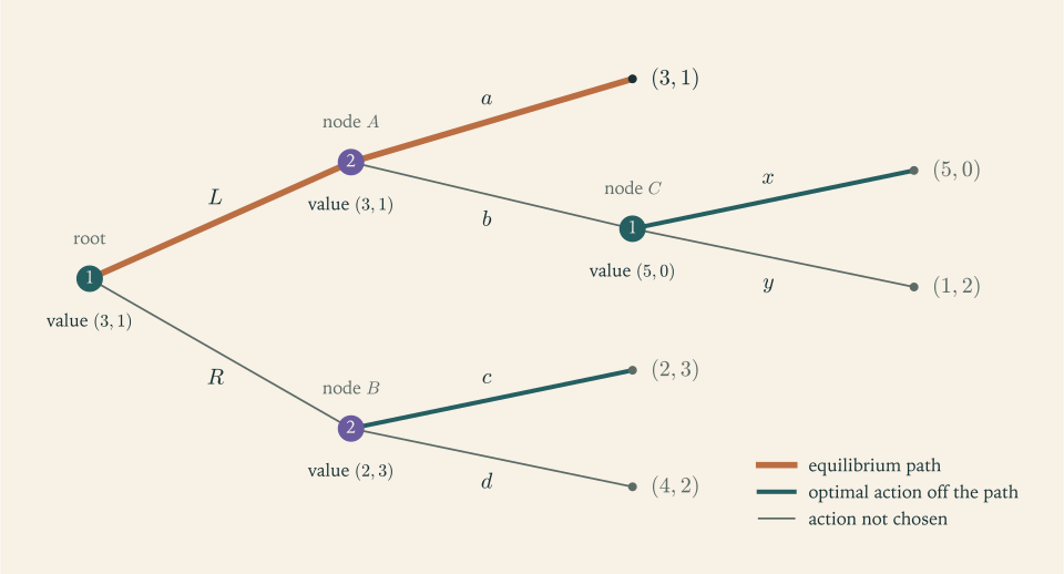
Look at the terminal node after \(R\) and \(d\) , with payoffs \((4,2)\) . Both players prefer it to the outcome \((3,1)\) . It is not reached because player 2, once at \(B\) , would choose \(c\) , and player 1, foreseeing that, does not choose \(R\) . Player 2 would be better off without the option \(c\) : if \(c\) were removed from the tree, player 1 would choose \(R\) and player 2 would get \(2\) instead of \(1\) . Having fewer options can help a player in a game, because it changes what others expect; in a decision problem with one decision maker that could never happen.
5.3 A leader and a follower
Backward induction does not need the tree to be finite in width. If the mover at some node chooses from a continuum, the procedure still works provided each choice problem has a solution.
Example 5.3: Stackelberg quantity leadership
Return to the two firms of Example 2.3, with price \(14-Q\) and unit cost \(2\) , but let firm 1 choose its quantity \(q_1\) first and let firm 2 observe \(q_1\) before choosing \(q_2\) . A strategy of firm 1 is a number \(q_1\) . A strategy of firm 2 is a function that gives a quantity for every possible \(q_1\) .
The follower. After any \(q_1\le 12\) , firm 2 maximizes \(q_2(12-q_1-q_2)\) , so its optimal choice is the reaction function of Chapter 2, \(q_2=(12-q_1)/2\) .
The leader. Anticipating this, firm 1’s profit as a function of \(q_1\) alone is
which is maximized at \(q_1=6\) . Then \(q_2=3\) , total output is \(9\) , the price is \(5\) , and the profits are \(6\cdot 3=18\) for the leader and \(3\cdot 3=9\) for the follower.
Compare the simultaneous game, where each firm produced \(4\) and earned \(16\) . The leader produces more and earns more; the follower produces less and earns less; and total output is higher. Firm 1 does not have better technology or information than before. It gains because it moves first and its choice is observed: it can commit to a large quantity, and the follower’s best reply to a large quantity is a small one. Notice also that the leader does not play a best response to the follower’s quantity: against \(q_2=3\) the best response would be \(4.5\) . The leader optimizes against the follower’s strategy, the whole reaction function, and moves along it.
5.4 Games that someone must win
In a game where two players move alternately, every play ends, and the only outcomes are a win for one or the other, Theorem 5.3 has a striking consequence.
Corollary 5.4 (determinacy). In a finite two-player extensive game with perfect information in which every terminal node is a win for one player and a loss for the other, exactly one of the players has a strategy that wins against every strategy of the opponent. If draws are also possible, then either one player has such a winning strategy or both players have strategies that guarantee at least a draw.
Proof. Assign the payoffs \(1\) for a win, \(0\) for a draw, and \(-1\) for a loss, and let \(s^\star\) be a backward-induction profile with outcome payoff \(v\) for player 1. By Theorem 5.3, \(s^\star\) is a Nash equilibrium of a zero-sum game, so player 1’s strategy guarantees player 1 at least \(v\) against every strategy of player 2, since player 2 has no deviation that lowers it, and player 2’s strategy holds player 1 to at most \(v\) . If \(v=1\) , player 1 has a winning strategy; if \(v=-1\) , player 2 has; if \(v=0\) , each can guarantee a draw. The cases exclude one another.
The corollary says that such games are, in principle, completely solved: before the first move one of the three verdicts is already true. For chess nobody knows which. For small games the verdict can be computed.
Example 5.4: Taking stones
A pile contains \(10\) stones. Two players alternately remove one or two stones, and whoever takes the last stone wins. Call a pile size losing if the player about to move loses when both play optimally, and winning otherwise. Backward induction on the pile size:
A pile of \(0\) is losing for the player to move, who has just seen the opponent take the last stone. A pile of \(1\) or \(2\) is winning: take everything. A pile of \(3\) is losing, because either move leaves \(2\) or \(1\) , a winning pile for the opponent. A pile of \(4\) or \(5\) is winning: remove \(1\) or \(2\) to leave \(3\) . A pile of \(6\) is losing, since both moves leave a winning pile. Continuing, the labels for the sizes \(0\) through \(10\) are
The losing piles are exactly the multiples of \(3\) . The general statement is proved by induction: from a multiple of \(3\) every move leaves a pile that is not a multiple of \(3\) , and from a pile that is not a multiple of \(3\) one can remove its remainder, \(1\) or \(2\) , to leave a multiple of \(3\) .
With \(10\) stones the first player wins: take \(1\) to leave \(9\) , and thereafter answer a removal of \(k\) stones by removing \(3-k\) . The winning strategy is a complete plan, specifying a reply at every pile size that can arise, and its description as a rule is far shorter than the tree, which has \(232\) nodes, \(89\) of them terminal.
5.5 When the backward-induction answer is hard to believe
Backward induction asks more of the players than it seems to. At each node the mover must expect all later movers to choose as the procedure says, and that expectation must be maintained even at nodes that could only have been reached if someone had already failed to choose as the procedure says.
Example 5.5: A centipede
Two players alternate, starting with player 1, at four decision nodes. At each node the mover can Stop, ending the game, or Continue. The payoffs if the game is stopped at the first, second, third, or fourth node are \((1,0)\) , \((0,2)\) , \((3,1)\) , and \((2,4)\) , and if nobody stops they are \((5,3)\) .
At the fourth node player 2 compares \(4\) from Stop with \(3\) from Continue and stops. At the third node player 1 compares \(3\) from Stop with \(2\) , the result of continuing and being stopped, and stops. At the second node player 2 compares \(2\) with \(1\) and stops. At the first node player 1 compares \(1\) with \(0\) and stops. By Theorem 5.3(b) this is the unique backward-induction profile: everybody stops at every node, and the outcome is \((1,0)\) .
Both players would prefer the game to reach the third node, or the fourth, or the end. Each stops because the other would stop one step later. The logic is the same as in Example 5.2, but here the prediction is uncomfortable, and people asked to play such games usually continue for a while. One way to see the difficulty: suppose player 1 continues at the first node. Player 2, now at the second node, has just watched player 1 do something that backward induction says player 1 would never do. Should player 2 still be certain that player 1 will stop at the third node? The procedure says yes, and offers no account of the evidence to the contrary. Backward induction describes what follows from common knowledge of rationality at every node, reached or not; it does not claim that this assumption survives being contradicted. The example does not show that the method is wrong, only that its conclusion is as strong as that assumption and no stronger.
Common mistake. Writing a strategy as a path. In Example 5.2 the answer “player 1 plays \(L\) , player 2 plays \(a\) ” describes the outcome, not a strategy profile. It does not say what player 2 would do at \(B\) or what player 1 would do at \(C\) , and without that information it is impossible to check whether \(L\) and \(a\) are optimal. Player 1’s strategy must name an action at the root and an action at \(C\) , even though choosing \(L\) and then seeing \(a\) means that \(C\) is not reached. An answer to “find the backward-induction solution” lists one action for every decision node in the tree, and then, separately, the outcome.
5.6 Moves that are not observed
Many games are sequential in time but not in information. Two firms may submit sealed bids on different days; the second bidder moves later but knows nothing that the first did. To represent such situations in a tree, nodes that a player cannot tell apart are grouped together.
Definition 5.5 (information sets). An extensive game with imperfect information is specified like the game of Definition 5.1, together with a partition of each player’s decision nodes into information sets, such that the same actions are available at every node of an information set. When play reaches a node, the player who moves there is told only which information set contains it. A strategy of player \(i\) assigns one action to each of player \(i\) ’s information sets. The game has perfect information when every information set is a single node.
A strategy must choose the same action at all nodes of an information set, because the player cannot make the choice depend on something the player does not know. We assume throughout that players remember what they themselves knew and did earlier, a condition called perfect recall. Chance events, such as a deal of cards, are included by adding a player called Nature who moves with fixed probabilities and has no payoffs; Chapters 7 and 8 use this device.
Example 5.6: What an information set changes
Take the seminar game of Example 2.2 and suppose player 1 chooses first.
If player 2 observes the choice, the game has perfect information. Player 2 has two decision nodes and \(4\) strategies, of the form “after Algebra do this, after Biology do that”. Backward induction: after Algebra, player 2 chooses Algebra (\(1>0\) ); after Biology, player 2 chooses Biology (\(2>0\) ); so player 1 compares \(2\) from Algebra with \(1\) from Biology and chooses Algebra. The outcome is (Algebra, Algebra) with payoffs \((2,1)\) . Moving first is an advantage here: player 1 gets the equilibrium that player 1 prefers.
If player 2 does not observe the choice, player 2’s two decision nodes form one information set. Player 2 has only \(2\) strategies, Algebra or Biology, and the strategic form is the \(2\times 2\) table of Chapter 2, with its three equilibria. Backward induction cannot begin: at player 2’s information set the best action depends on which node has been reached, and player 2 does not know.
The physical order of moves is the same in the two versions. What differs is what player 2 knows when choosing, and that is what determines the strategy sets and the solution. A simultaneous-move game is one in which each player moves at a single information set without having observed anything.
So the method of this chapter has a clear domain. With perfect information it selects, among the Nash equilibria, those whose plans are optimal at every node. For trees with information sets it stalls at the first node it cannot isolate. Chapter 6 extends the idea as far as it will go by applying it to those parts of a tree that can be isolated, and Chapter 8 handles the rest by adding to the description of an equilibrium the players’ beliefs about where they are.
Exercises
-
In a game tree, player 1 moves at the root with three actions; after each of them player 2 moves with two actions; after each of player 2’s actions player 1 moves again with two actions, and then the game ends. How many decision nodes does each player have, how many strategies does each player have, and how many terminal nodes are there? Write out one complete strategy of player 1 in words.
Answer
Player 1 has \(1+6=7\) decision nodes and \(3\cdot 2^6=192\) strategies; player 2 has \(3\) decision nodes and \(2^3=8\) strategies; there are \(3\cdot 2\cdot 2=12\) terminal nodes. A strategy of player 1 names an action at the root and one action at each of the six later nodes, for example: “the first action at the root, and the first action at every later node, whichever of them is reached”.
-
Player 1 chooses \(A\) or \(B\) . After \(A\) , player 2 chooses \(c\) , with payoffs \((2,2)\) , or \(d\) , with payoffs \((0,3)\) . After \(B\) , player 2 chooses \(e\) , with payoffs \((3,1)\) , or \(f\) , after which player 1 chooses \(g\) , with payoffs \((1,0)\) , or \(h\) , with payoffs \((4,4)\) . Find the backward-induction profile, listing an action at every decision node, and the outcome.
Solution
Work from the end. At player 1’s last node, after \(B\) and \(f\) , the choice is between \(1\) from \(g\) and \(4\) from \(h\) : choose \(h\) , and the node is worth \((4,4)\) . At player 2’s node after \(B\) , the choice is between \(1\) from \(e\) and \(4\) from \(f\) (which leads to \((4,4)\) ): choose \(f\) , and the node is worth \((4,4)\) . At player 2’s node after \(A\) , the choice is between \(2\) from \(c\) and \(3\) from \(d\) : choose \(d\) , and the node is worth \((0,3)\) . At the root player 1 compares \(0\) from \(A\) with \(4\) from \(B\) : choose \(B\) .
The backward-induction profile is: player 1 plays \(B\) at the root and \(h\) at the last node; player 2 plays \(d\) after \(A\) and \(f\) after \(B\) . The outcome is \(B\) , \(f\) , \(h\) with payoffs \((4,4)\) . No player is indifferent between any two terminal nodes, so by Theorem 5.3(b) this profile is the only one.
-
For the game of the previous exercise, write the \(4\times 4\) strategic form, find all pure Nash equilibria, and for each equilibrium that is not the backward-induction profile identify a node at which the prescribed action is not optimal.
Solution
Player 1’s strategies are \(Ag,Ah,Bg,Bh\) (root action, then action at the last node) and player 2’s are \(ce,cf,de,df\) (action after \(A\) , then action after \(B\) ):
\[ \begin{array}{c|cccc} & ce & cf & de & df\\ \hline Ag & (2,2) & (2,2) & (0,3) & (0,3)\\ Ah & (2,2) & (2,2) & (0,3) & (0,3)\\ Bg & (3,1) & (1,0) & (3,1) & (1,0)\\ Bh & (3,1) & (4,4) & (3,1) & (4,4) \end{array} \]Marking best responses, player 1’s best payoffs in the four columns are \(3\) (rows \(Bg\) , \(Bh\) ), \(4\) (row \(Bh\) ), \(3\) (rows \(Bg\) , \(Bh\) ), and \(4\) (row \(Bh\) ). Player 2’s best payoffs in the rows are \(3\) (columns \(de\) , \(df\) ) for \(Ag\) and \(Ah\) , \(1\) (columns \(ce\) , \(de\) ) for \(Bg\) , and \(4\) (columns \(cf\) , \(df\) ) for \(Bh\) . There are four pure Nash equilibria: \((Bg,ce)\) , \((Bg,de)\) , \((Bh,cf)\) , and \((Bh,df)\) .
Only \((Bh,df)\) is the backward-induction profile. In \((Bg,ce)\) and \((Bg,de)\) player 1 plans \(g\) at the last node, which yields \(1\) where \(h\) yields \(4\) ; the plan is a threat against player 2’s choice of \(f\) , and it makes player 2 choose \(e\) , so the outcome is \((3,1)\) instead of \((4,4)\) . The threat hurts both players and is never carried out. In \((Bh,cf)\) , player 2 plans \(c\) after \(A\) , which yields \(2\) where \(d\) yields \(3\) ; this node is not reached, and the outcome is the same as under backward induction, but the plan is still not optimal there. In \((Bg,ce)\) the action \(c\) is not optimal either.
-
Prove that a player who moves at \(k\) nodes with \(m_1,\dots,m_k\) available actions has \(m_1m_2\cdots m_k\) strategies. Then explain why two strategies of that player that differ only at a node the player’s own earlier action excludes always produce the same outcome, and why Definition 5.2 nevertheless counts them as different.
Hint
A strategy is one choice from each of \(k\) independent lists, so the product rule of counting applies. Two strategies that differ only at a node excluded by the player’s own earlier action lead to the same path whatever the opponents do. They are different functions on the set of the player’s nodes, and the definition keeps them apart because the action at the excluded node is what the other players reason about when they ask what would happen if the player had acted differently.
-
Solve the Stackelberg game with price \(20-Q\) and unit cost \(2\) for both firms: give the follower’s strategy, the leader’s quantity, the price, and both profits, and compare with the simultaneous-move outcome.
Answer
Follower: \(q_2=(18-q_1)/2\) . Leader: maximize \(q_1(18-q_1)/2\) , so \(q_1=9\) and \(q_2=4.5\) . Price \(6.5\) ; profits \(40.5\) and \(20.25\) . In the simultaneous game each firm produces \(6\) , the price is \(8\) , and each earns \(36\) .
-
Two firms sell differentiated products at zero cost; firm \(i\) sells \(12-2p_i+p_j\) units. Firm 1 sets its price first and firm 2 observes it. Find the backward-induction prices and profits. Which firm earns more, and how do both profits compare with the simultaneous-move profits of \(32\) each?
Solution
The follower. Given \(p_1\) , firm 2 maximizes \(p_2(12-2p_2+p_1)\) , a concave quadratic in \(p_2\) with derivative \(12-4p_2+p_1\) , so \(p_2=(12+p_1)/4\) .
The leader. Substituting, firm 1’s sales are \(12-2p_1+(12+p_1)/4=15-\tfrac74p_1\) , and its profit is \(p_1(15-\tfrac74p_1)\) , with derivative \(15-\tfrac72p_1\) . Hence \(p_1=30/7\approx 4.29\) , and then \(p_2=(12+\tfrac{30}{7})/4=57/14\approx 4.07\) .
Profits. Firm 1 earns \(\tfrac{30}{7}\cdot(15-\tfrac{15}{2})=225/7\approx 32.14\) . For firm 2, the first-order condition says \(12+p_1=4p_2\) , so its sales are \(12-2p_2+p_1=2p_2\) and its profit is \(2p_2^2=2\cdot\tfrac{3249}{196}=3249/98\approx 33.15\) .
The follower earns more than the leader, and both earn more than the \(32\) of the simultaneous game. With prices, a higher price by one firm makes the other want a higher price too. The leader commits to a price above the simultaneous level, which softens competition; the follower then undercuts it slightly and gains the most. In the quantity game of Example 5.3 the reaction function slopes the other way and the advantage goes to the first mover.
-
A pile has \(21\) stones; two players alternately remove one, two, or three stones, and whoever takes the last stone wins. Determine all losing pile sizes, prove your claim by induction, and state the first player’s winning strategy.
Solution
Claim. A pile of \(n\) stones is losing for the player about to move if and only if \(n\) is a multiple of \(4\) .
Proof by strong induction on \(n\) . A pile of \(0\) is losing: the previous player took the last stone. Let \(n\ge 1\) and suppose the claim holds for all smaller piles. If \(n\) is not a multiple of \(4\) , let \(r\in\{1,2,3\}\) be its remainder on division by \(4\) . Removing \(r\) stones is a legal move and leaves a multiple of \(4\) , which by the induction hypothesis is losing for the opponent; so \(n\) is winning. If \(n\) is a multiple of \(4\) , any legal move removes \(1\) , \(2\) , or \(3\) stones and leaves a pile that is not a multiple of \(4\) , which by hypothesis is winning for the opponent; so \(n\) is losing.
The losing piles are the multiples of \(4\) : \(0,4,8,12,16,20\) among sizes up to \(21\) . Since \(21=4\cdot 5+1\) , the first player wins. The winning strategy: take \(1\) stone, leaving \(20\) ; thereafter, whenever the opponent removes \(k\) stones, remove \(4-k\) . After each such pair of moves the pile is again a multiple of \(4\) , so the first player eventually takes the last stone.
-
In the centipede of Example 5.5, change the payoff after the fourth node’s Continue from \((5,3)\) to \((5,6)\) . Redo the backward induction, and explain why changing one terminal payoff alters the action at every node.
Answer
Now player 2 continues at the fourth node (\(6>4\) ), so that node is worth \((5,6)\) ; player 1 continues at the third (\(5>3\) ); player 2 at the second (\(6>2\) ); player 1 at the first (\(5>1\) ). Everyone continues and the outcome is \((5,6)\) . Each node’s value is computed from the value of the next one, so a change at the end propagates all the way back.
-
A proposer offers a responder a whole number \(x\in\{0,1,\dots,10\}\) of ten coins; the responder accepts, giving payoffs \((10-x,x)\) , or rejects, giving \((0,0)\) . Find all backward-induction profiles. Then exhibit a Nash equilibrium in which the coins are split equally, and say why it is not a backward-induction profile.
Solution
The responder. At the node after an offer \(x\ge 1\) , accepting gives \(x>0\) and rejecting gives \(0\) , so the responder accepts. After the offer \(x=0\) both actions give \(0\) : the responder is indifferent, and backward induction branches.
Branch 1: the responder accepts \(0\) . Then every offer is accepted, the proposer’s payoff from \(x\) is \(10-x\) , and the proposer offers \(x=0\) . Outcome \((10,0)\) .
Branch 2: the responder rejects \(0\) . Then the proposer gets \(0\) from offering \(0\) and \(10-x\) from any \(x\ge 1\) , and offers \(x=1\) . Outcome \((9,1)\) .
There are exactly two backward-induction profiles: (offer \(0\) ; accept everything) and (offer \(1\) ; accept exactly the offers \(x\ge 1\) ).
An equal split as a Nash equilibrium. Let the responder’s strategy be “accept if \(x\ge 5\) , reject otherwise” and let the proposer offer \(5\) . The proposer gets \(5\) ; a lower offer is rejected and gives \(0\) ; a higher offer is accepted and gives less than \(5\) . The responder gets \(5\) ; no other strategy gives more against the offer \(5\) . So this is a Nash equilibrium with outcome \((5,5)\) . It is not a backward-induction profile because the responder’s plan rejects the offers \(1\) through \(4\) , and at each of those nodes rejecting yields \(0\) where accepting yields a positive amount. The equal split is sustained by a threat that would not be carried out.
-
A student answers Example 5.2 with “Player 1’s strategy is \(L\) . The action at \(C\) is irrelevant because \(C\) is never reached.” Explain what is missing from the strategy, and show by changing player 1’s action at \(C\) to \(y\) that the action there affects whether \((L,a)\) can be the outcome of an equilibrium.
Hint
A strategy for player 1 needs an action at the root and one at \(C\) . Suppose player 1’s action at \(C\) were \(y\) . Then \(b\) would lead to \((1,2)\) , and player 2 at \(A\) would compare \(1\) from \(a\) with \(2\) from \(b\) . What would player 2 choose, and what would player 1 then get from \(L\) ?
-
For the version of Example 5.6 in which player 2 observes player 1’s choice, write the \(2\times 4\) strategic form, find all pure Nash equilibria, and say which one is the backward-induction profile.
Answer
Write player 2’s strategies as pairs (reply to Algebra, reply to Biology). The row Algebra gives \((2,1)\) against the two strategies that reply Algebra to Algebra and \((0,0)\) against the others; the row Biology gives \((1,2)\) against the two strategies that reply Biology to Biology and \((0,0)\) against the others. The pure Nash equilibria are: Algebra with (Algebra, Algebra); Algebra with (Algebra, Biology); and Biology with (Biology, Biology). The backward-induction profile is Algebra with (Algebra, Biology). In the third equilibrium player 2 threatens to go to Biology even after seeing Algebra, which would give \(0\) instead of \(1\) .
-
In matching pennies let player 1 choose first and player 2 observe the choice. Find the backward-induction outcome and compare player 1’s payoff with the maximizer’s security level in pure strategies and with the value of the simultaneous game from Chapter 4.
Answer
Player 2 observes and mismatches, so player 1 gets \(-1\) whichever side is shown. That equals the maximizer’s security level in pure strategies, \(-1\) , and is below the value \(0\) of the simultaneous game. Moving first in a zero-sum game means announcing a pure strategy, and the mover gets the pure maximin payoff.
-
Prove that in a finite two-player zero-sum extensive game with perfect information, the backward-induction payoff to player 1 equals the value of the strategic form, and that both players have pure optimal strategies.
Hint
By Theorem 5.3 the backward-induction profile is a pure Nash equilibrium of the strategic form, which is a matrix game. Apply Corollary 4.5(b): every equilibrium of a matrix game gives the maximizer the value. Then Corollary 4.5(a) says the two pure strategies are optimal.
-
Three firms decide in order, each observing the earlier decisions, whether to enter a market. A firm that stays out gets \(0\) ; an entrant gets \(6\) if it is alone, \(2\) if there are two entrants, and \(-1\) if there are three. Find the backward-induction profile, specifying firm 3’s action after each of the four possible histories, and the outcome.
Solution
Firm 3 moves last, knowing how many firms have entered. After two entries, entering gives \(-1\) and staying out gives \(0\) : stay out. After one entry (by either earlier firm), entering gives \(2\) : enter. After no entry, entering gives \(6\) : enter.
Firm 2. If firm 1 entered: entering leads to firm 3 staying out, so firm 2 gets \(2\) ; staying out leads to firm 3 entering, so firm 2 gets \(0\) . Enter. If firm 1 stayed out: entering leads to firm 3 entering as well, so firm 2 gets \(2\) ; staying out leads to firm 3 entering alone, so firm 2 gets \(0\) . Enter.
Firm 1. Entering leads to firm 2 entering and firm 3 staying out, for a payoff of \(2\) . Staying out leads to firms 2 and 3 both entering, for a payoff of \(0\) . Enter.
The backward-induction profile: firm 1 enters; firm 2 enters after either history; firm 3 stays out after two entries and enters after the other three histories. The outcome is that firms 1 and 2 enter and firm 3 stays out, with payoffs \((2,2,0)\) . The market has room for two, and the order of moves decides which two: the early movers commit, and the last mover adapts.
-
Describe rock–paper–scissors as an extensive game in which player 1 moves first and player 2 does not observe the move. How many information sets, decision nodes, and strategies does each player have? Explain why backward induction cannot be started.
Answer
Player 1 has one decision node, the root, which is its own information set, and \(3\) strategies. Player 2 has three decision nodes, one after each of player 1’s actions, all in a single information set, and therefore \(3\) strategies, not \(27\) . Backward induction would begin at player 2’s nodes, but the best action differs from node to node and player 2 cannot tell them apart.
-
Two players alternate moves, player 1 first; each player moves exactly twice, and three actions are available at every decision node. How many decision nodes and how many strategies does each player have? Give the exponent as well as the number.
Answer
Player 1 moves at the root and at the \(9\) nodes reached after two moves: \(10\) decision nodes and \(3^{10}=59049\) strategies. Player 2 moves at the \(3\) nodes after one move and the \(27\) nodes after three moves: \(30\) decision nodes and \(3^{30}\) strategies, about \(2\times 10^{14}\) .
-
In Example 5.2, suppose player 2 can, before the game starts and in full view of player 1, irreversibly remove one of her own four actions. Which action should she remove, and what are the resulting payoffs? Explain why the option she removes is one she would have used.
Hint
Try removing each of \(a\) , \(b\) , \(c\) , \(d\) in turn and redo the backward induction. Removing \(c\) makes player 1 choose \(R\) and gives \((4,2)\) . The removed action is the one player 2 would have chosen at \(B\) ; removing an action she would never choose changes nothing.
-
In the sequential game of Example 5.3, consider the profile in which firm 1 produces \(4\) and firm 2’s strategy is “produce \(4\) whatever \(q_1\) is”. Using the results of Chapter 2, show that this is a Nash equilibrium of the sequential game. Then show that it is not a backward-induction profile by naming a value of \(q_1\) after which firm 2’s prescribed quantity is not optimal.
Solution
It is a Nash equilibrium. Against firm 2’s strategy “produce \(4\) whatever \(q_1\) is”, firm 1 faces a rival quantity of \(4\) regardless of its own choice, so its problem is that of Chapter 2: maximize \(q_1(12-q_1-4)\) , solved by \(q_1=4\) . So firm 1’s quantity is a best response. Against \(q_1=4\) , firm 2’s payoff depends only on the quantity its strategy prescribes after \(q_1=4\) , and the best such quantity is the Cournot reply \((12-4)/2=4\) ; the constant strategy prescribes exactly that. So firm 2’s strategy is a best response, and the profile is a Nash equilibrium. Its outcome is the Cournot outcome \((4,4)\) with profits \(16\) each, not the Stackelberg outcome.
It is not a backward-induction profile. Take \(q_1=6\) . At the node after \(q_1=6\) firm 2’s optimal quantity is \((12-6)/2=3\) , which earns \(3\cdot 3=9\) , while the prescribed quantity \(4\) earns \(4\cdot(12-6-4)=8\) . The strategy is not optimal there, nor at any node other than the one after \(q_1=4\) . Firm 2’s constant strategy is a threat to ignore firm 1’s commitment; if firm 1 believed it, firm 1 would not try to lead. Backward induction discards it because firm 2 would in fact respond.