Every finite game examined in Chapter 3 turned out to have an equilibrium once mixed strategies were allowed. Three examples and a handful of exercises are not a theorem. Is there a finite game, perhaps with seven players and awkward payoffs, in which the best-response correspondences simply fail to meet? If there were, the equilibrium concept would be a tool that works on some games and is silent on others, and one would need to know in advance which kind one was facing.

There is no such game. Every finite game has at least one Nash equilibrium in mixed strategies. This chapter proves it twice. The first proof covers games of pure conflict between two players, where one side’s gain is the other’s loss; there the argument is constructive, the equilibrium is the solution of a linear program, and the equilibrium payoff is the same in every equilibrium. The second proof covers all finite games; it is not constructive, it rests on a fixed-point theorem, and it tells us nothing about how many equilibria there are. Seeing both, and seeing exactly which properties of the game each one uses, is the best protection against misapplying either.

4.1 Games of pure conflict

Here \(\Delta_m\) is the set of probability vectors with \(m\) coordinates. Player 1 wants \(x^{\top}Ay\) large and player 2 wants it small, and we shall call them the maximizer and the minimizer. A game in which the two payoffs always add up to the same constant, instead of to zero, is analysed in the same way, because subtracting a constant from one player’s payoffs changes no best response.

In such a game a cautious question has a clear meaning: how much can a player guarantee, without knowing anything about what the opponent will do?

The number \(\underline v\) is the largest payoff the maximizer can be sure of: whatever \(x\) is announced, the worst case is \(\min_yx^{\top}Ay\) , and \(\underline v\) is the best worst case. Likewise \(\overline v\) is the smallest ceiling the minimizer can impose. For a fixed \(x\) the function \(y\mapsto x^{\top}Ay\) is linear, so by Theorem 3.4(a), applied to the minimizer, its minimum over \(\Delta_n\) is reached at a pure strategy: \(\min_yx^{\top}Ay=\min_j(x^{\top}A)_j\) , the smallest coordinate of the row vector \(x^{\top}A\) . Similarly \(\max_xx^{\top}Ay=\max_i(Ay)_i\) . The inner optimizations are therefore finite comparisons. The outer ones are attained because a continuous function on a closed bounded subset of \(\mathbb R^m\) has a maximum and a minimum; closed bounded sets are compact by the Heine–Borel theorem (math.real-analysis.heine-borel).

The lemma says only that the two guarantees are compatible: the maximizer cannot be sure of more than the minimizer can be sure of conceding. The content of the theory is that they coincide.

Example 4.1: A penalty kick

A kicker aims Left or Right and, at the same moment, the goalkeeper dives Left or Right (both described from the kicker’s side). The kicker’s payoff is the probability of scoring and the goalkeeper’s is its negative:

\[ A=\begin{pmatrix}0.5&0.9\\0.8&0.3\end{pmatrix}, \]

with rows for the kicker’s Left and Right and columns for the goalkeeper’s Left and Right. The kicker is stronger to the left, scoring with probability \(0.9\) into an empty side there against \(0.8\) on the right.

In pure strategies. Kicking Left guarantees \(\min\{0.5,0.9\}=0.5\) and kicking Right guarantees \(\min\{0.8,0.3\}=0.3\) , so the kicker can guarantee \(0.5\) with a pure strategy. Diving Left concedes at most \(\max\{0.5,0.8\}=0.8\) and diving Right at most \(\max\{0.9,0.3\}=0.9\) , so the goalkeeper can hold the kicker to \(0.8\) . There is a gap between \(0.5\) and \(0.8\) , and no pure equilibrium.

In mixed strategies. Let the kicker aim Left with probability \(p\) . Against a dive Left the scoring probability is \(0.5p+0.8(1-p)=0.8-0.3p\) , and against a dive Right it is \(0.9p+0.3(1-p)=0.3+0.6p\) . The kicker’s guarantee is the smaller of the two, a function of \(p\) that rises along the second line and then falls along the first. Its maximum is where the lines cross: \(0.8-0.3p=0.3+0.6p\) gives \(p=5/9\) , and the guarantee there is \(0.8-0.3\cdot\tfrac59=\tfrac{19}{30}\approx 0.633\) .

Let the goalkeeper dive Left with probability \(q\) . A kick Left scores with probability \(0.5q+0.9(1-q)=0.9-0.4q\) and a kick Right with probability \(0.8q+0.3(1-q)=0.3+0.5q\) . The goalkeeper’s ceiling is the larger of the two, and it is smallest where they cross: \(0.9-0.4q=0.3+0.5q\) gives \(q=2/3\) , with ceiling \(0.9-0.4\cdot\tfrac23=\tfrac{19}{30}\) .

So \(\underline v=\overline v=19/30\) . By mixing, the kicker raises the guarantee from \(0.5\) to about \(0.633\) and the goalkeeper lowers the ceiling from \(0.8\) to the same number. The kicker aims at the stronger side only slightly more than half the time; the goalkeeper covers that side two thirds of the time.

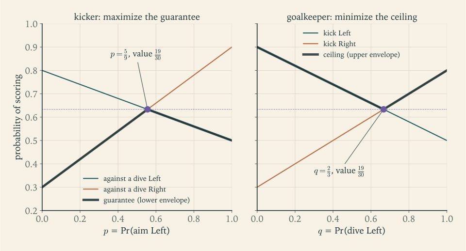
Figure 4.1 shows why the optimum sits at a kink. To the left of \(p=5/9\) the binding threat is a dive Right, and increasing \(p\) helps against it; to the right the binding threat is a dive Left, and increasing \(p\) hurts. At the kink both of the goalkeeper’s pure strategies are equally good replies, which is the indifference principle seen from the other side.

4.2 The minimax theorem

The proof converts the two guarantees into a pair of linear programs that are dual to each other. The fact imported is strong duality: if a linear program in the standard form “minimize \(c^{\top}z\) subject to \(Mz=b\) , \(z\ge 0\) ” has an optimal solution, then so does its dual “maximize \(b^{\top}\eta\) subject to \(M^{\top}\eta\le c\) ”, and the two optimal values are equal (math.continuous-optimization.linear-programming-vertices-duality).

The proof is also a method. To solve a matrix game numerically one solves the maximizer’s program directly, without the change of variables: maximize \(v\) over \((x,v)\) subject to \((x^{\top}A)_j\ge v\) for every column \(j\) , \(\mathbf 1^{\top}x=1\) , and \(x\ge 0\) . The minimizer’s program is: minimize \(w\) subject to \((Ay)_i\le w\) for every row \(i\) , \(\mathbf 1^{\top}y=1\) , and \(y\ge 0\) .

Zero-sum games are thus exceptionally well behaved. An equilibrium exists; all equilibria have the same payoff; a player need not know which equilibrium the opponent has in mind, since any optimal strategy is in equilibrium with any optimal strategy of the opponent; and equilibrium strategies are exactly the cautious ones. None of these properties survives in general games. In the seminar game of Chapter 3 the three equilibria have three different payoff pairs, and combining player 1’s strategy from one pure equilibrium with player 2’s from the other gives a profile where both get \(0\) .

4.3 General games: equilibrium as a fixed point

Outside the zero-sum world there are no security levels to equate. The maximin payoff of a player in a general game says what that player can guarantee, but equilibrium payoffs can be higher, and equilibrium strategies need not be cautious. A different idea is needed, and it comes from rewriting the definition.

Let \(G\) be a finite game, and let \(\Sigma=\Delta(S_1)\times\dots\times\Delta(S_n)\) be the set of mixed profiles. For \(\sigma\in\Sigma\) let \(B_i(\sigma)\subseteq\Delta(S_i)\) be the set of mixed best responses of player \(i\) to \(\sigma_{-i}\) , and put

This is the best-response correspondence of the game: it assigns to each profile the set of profiles in which everybody is best-responding to it. By Proposition 2.2, applied to the mixed extension,

An equilibrium is a fixed point of \(B\) . Existence of equilibrium is existence of a fixed point for a set-valued map, and for that there is a classical theorem. We state it with all its hypotheses, because each one will have to be verified.

Kakutani’s fixed-point theorem: let \(X\) be a nonempty, compact, convex subset of \(\mathbb R^d\) , and let \(F\) assign to each \(x\in X\) a subset \(F(x)\subseteq X\) such that (i) \(F(x)\) is nonempty for every \(x\) , (ii) \(F(x)\) is convex for every \(x\) , and (iii) the graph \(\{(x,y):y\in F(x)\}\) is a closed subset of \(X\times X\) . Then there is a point \(x^\star\in X\) with \(x^\star\in F(x^\star)\) (math.functional-analysis.kakutani-fixed-point). Condition (iii) says that if \(x^k\to x\) , \(y^k\to y\) , and \(y^k\in F(x^k)\) for all \(k\) , then \(y\in F(x)\) . When \(F(x)\) is always a single point, (iii) says that \(F\) is a continuous function, (ii) is automatic, and the statement is Brouwer’s fixed-point theorem.

Notice where mixed strategies entered. Compactness and nonemptiness would hold equally for the finite sets \(S_i\) . Convexity of the strategy sets, and convexity of the sets of best responses, are what randomization supplies. Without them the theorem is false, as matching pennies shows.

4.4 What each hypothesis is for

A theorem is understood when one knows what goes wrong without each assumption. Nash’s theorem assumes finitely many players, finitely many pure strategies, and mixed strategies with expected payoffs. The more general result below makes the role of each property explicit.

Theorem 4.7 is the special case in which the strategy sets are simplices and the payoffs are expected payoffs, linear and hence quasi-concave in a player’s own mixture. Theorem 4.8 also covers games that were solved in Chapter 2 by calculus, and games that cannot be solved in closed form at all.

4.5 Symmetric games

Many games treat the players alike: the Cournot duopoly with equal costs, the volunteer’s dilemma, hawk–dove. A two-player game is symmetric if \(S_1=S_2\) and \(u_2(s_1,s_2)=u_1(s_2,s_1)\) for all \(s_1,s_2\) ; in a table, player 2’s payoff matrix is the transpose of player 1’s. In such games it is natural to look for equilibria in which both players do the same thing, as we did in Example 3.6.

The theorem does not say that every equilibrium of a symmetric game is symmetric. Hawk–dove has two asymmetric pure equilibria, in which one animal is the hawk and the other the dove, and one symmetric mixed equilibrium. The symmetric one is the relevant prediction when the players cannot tell their roles apart, as in a population where an animal does not know whether it is “player 1”. The same argument works for \(n\) players, and for games with continuous strategy sets that satisfy the hypotheses of Theorem 4.8.

The games met so far were all played in a single simultaneous move. Existence is now settled for them, and the next four chapters turn to what the strategic form hides: the order of moves, the credibility of threats, and private information. Each will produce games with many Nash equilibria, most of which are unreasonable, and the work will be to say which and why.

Exercises

1. For the matrix game \(\begin{pmatrix}3&1&4\\2&0&1\\5&1&6\end{pmatrix}\) compute the maximizer’s and the minimizer’s security levels in pure strategies, find every pure equilibrium, and state the value of the game.

   Answer

   Row minima are \(1,0,1\) , so the maximizer’s pure security level is \(1\) . Column maxima are \(5,1,6\) , so the minimizer’s is \(1\) . They agree; the pure equilibria are the entries equal to \(1\) that are smallest in their row and largest in their column, namely (row 1, column 2) and (row 3, column 2). The value is \(1\) .

2. Solve the matrix game \(\begin{pmatrix}2&-1\\-3&4\end{pmatrix}\) : find both optimal mixed strategies and the value, and present the certificate that proves optimality.

   Answer

   \(x^\star=(\tfrac{7}{10},\tfrac{3}{10})\) , \(y^\star=(\tfrac12,\tfrac12)\) , \(v=\tfrac12\) . Certificate: \((x^\star)^{\top}A=(1.4-0.9,\ -0.7+1.2)=(0.5,0.5)\) and \(Ay^\star=(1-0.5,\ -1.5+2)=(0.5,0.5)\) .

3. In the matrix game \(\begin{pmatrix}1&4&2\\5&1&3\end{pmatrix}\) the maximizer has two rows. Plot or tabulate the three lines that give the maximizer’s payoff against each column as a function of the probability \(p\) of the first row, find the maximin strategy and the value, determine which column the minimizer never uses, and find the minimizer’s optimal strategy.

   Solution

   Let the maximizer play row 1 with probability \(p\) . The payoffs against the three columns are

   \[ p+5(1-p)=5-4p,\qquad 4p+(1-p)=1+3p,\qquad 2p+3(1-p)=3-p . \]

   At \(p=0\) they are \(5,1,3\) and at \(p=1\) they are \(1,4,2\) . The guarantee is the lower envelope of the three lines. The second and third lines cross at \(1+3p=3-p\) , that is, \(p=\tfrac12\) , where both equal \(2.5\) and the first line equals \(3\) . For \(p<\tfrac12\) the smallest line is \(1+3p\) , which is increasing; for \(p>\tfrac12\) the smallest is \(3-p\) until it meets \(5-4p\) at \(p=\tfrac23\) , and both of those are decreasing. So the envelope rises until \(p=\tfrac12\) and falls afterwards: the maximin strategy is \(x=(\tfrac12,\tfrac12)\) and the value is \(2.5\) .

   At the optimum the first column gives the maximizer \(3>2.5\) , so the minimizer never uses it. With probability \(y\) on column 2 and \(1-y\) on column 3, the two rows earn \(4y+2(1-y)=2+2y\) and \(y+3(1-y)=3-2y\) ; equality gives \(y=\tfrac14\) . So \(y=(0,\tfrac14,\tfrac34)\) .

   Certificate: \(x^{\top}A=(3,\ 2.5,\ 2.5)\) , all at least \(2.5\) , and \(Ay=(2.5,\ 2.5)\) , all at most \(2.5\) .

4. Let \(f(x,y)\) be any real function on a product of finite sets \(X\times Y\) . Prove that \(\max_x\min_yf(x,y)\le\min_y\max_xf(x,y)\) , and give a \(2\times 2\) example in which the inequality is strict.

   Solution

   Let \(\hat x\) attain the outer maximum on the left and \(\hat y\) the outer minimum on the right. Then

   \[ \max_x\min_yf(x,y)=\min_yf(\hat x,y)\le f(\hat x,\hat y)\le\max_xf(x,\hat y)=\min_y\max_xf(x,y). \]

   The first inequality holds because a minimum over \(y\) is at most the value at the particular point \(\hat y\) , and the second because a maximum over \(x\) is at least the value at \(\hat x\) . Finiteness of \(X\) and \(Y\) guarantees that the maxima and minima exist.

   For a strict inequality take matching pennies, \(f(H,H)=f(T,T)=1\) and \(f(H,T)=f(T,H)=-1\) . Each row has minimum \(-1\) , so the left side is \(-1\) . Each column has maximum \(1\) , so the right side is \(1\) . Whoever must commit first loses; the gap is the value of knowing the other’s choice.

5. Let the matrix game \(A\) have value \(v\) . Prove that for \(k>0\) and any real \(c\) the game with matrix \(kA+c\) (every entry multiplied by \(k\) and increased by \(c\) ) has value \(kv+c\) and the same optimal strategies.

   Hint

   For probability vectors, \(x^{\top}(kA+c)y=k\,x^{\top}Ay+c\) , because the entries of \(x\) and of \(y\) each sum to one. Multiplying by \(k>0\) and adding \(c\) preserves every inequality in Theorem 4.4.

6. A matrix game is symmetric if \(A^{\top}=-A\) . Prove that the value of a symmetric matrix game is \(0\) . Then find an optimal strategy for the variant of rock–paper–scissors with matrix \(\begin{pmatrix}0&-1&2\\1&0&-1\\-2&1&0\end{pmatrix}\) , in which rock beating scissors counts double, and explain why paper is played most.

   Solution

   The value is zero. For any vector \(x\) , the number \(x^{\top}Ax\) equals its own transpose \(x^{\top}A^{\top}x=-x^{\top}Ax\) , so \(x^{\top}Ax=0\) . In a symmetric game both players have the same number of strategies, so any \(x\in\Delta_m\) may be used by either. For any maximizer strategy \(x\) , the minimizer can reply with \(y=x\) , so \(\min_yx^{\top}Ay\le 0\) and hence \(\underline v\le 0\) . For any minimizer strategy \(y\) , the maximizer can reply with \(x=y\) , so \(\max_xx^{\top}Ay\ge 0\) and \(\overline v\ge 0\) . By the minimax theorem \(\underline v=\overline v\) , so both are \(0\) .

   The variant of rock–paper–scissors. An optimal \(x\) must earn at least \(0\) against every column. Try to make all three equal to \(0\) : the columns give \(x_2-2x_3=0\) , \(-x_1+x_3=0\) , and \(2x_1-x_2=0\) . So \(x_3=x_1\) and \(x_2=2x_1\) , and with \(x_1+x_2+x_3=1\) we get \(x=(\tfrac14,\tfrac12,\tfrac14)\) . It earns \((0,0,0)\) against the columns, so it guarantees the value \(0\) and is optimal; by symmetry the same strategy is optimal for the minimizer.

   Paper is played most because rock has become more attractive, its win being worth double, and paper is what beats rock. In equilibrium the popularity of a strategy reflects the payoff of the strategy it defeats, a version of the principle that a player’s mixture is tuned to the opponent’s incentives.

7. A commentator says of Example 4.1: “The kicker scores with probability \(0.9\) on the left against \(0.8\) on the right, so he should always go left.” Compute what the kicker gets from that plan once the goalkeeper anticipates it, compare with the value, and explain what the commentator’s argument ignores.

   Answer

   A goalkeeper who expects Left dives Left, and the kicker scores with probability \(0.5\) , below the value \(19/30\approx 0.633\) . The commentator compared the two best cases for the kicker, in which the goalkeeper guesses wrong, and ignored that the goalkeeper’s choice responds to the kicker’s plan.

8. Write the maximizer’s linear program for the matrix game \(\begin{pmatrix}0&1&1\\-3&2&0\\4&0&1\end{pmatrix}\) , and verify by a certificate that \(x=(\tfrac12,\tfrac16,\tfrac13)\) and \(y=(\tfrac16,\tfrac23,\tfrac16)\) are optimal. What is the value?

   Solution

   The maximizer’s program has variables \(x_1,x_2,x_3,v\) :

   \[ \begin{aligned} \text{maximize}\quad & v\\ \text{subject to}\quad & -3x_2+4x_3\ge v,\quad x_1+2x_2\ge v,\quad x_1+x_3\ge v,\\ & x_1+x_2+x_3=1,\quad x_1,x_2,x_3\ge 0 . \end{aligned} \]

   There is one inequality for each column, obtained by reading down that column of the matrix.

   Certificate for \(x=(\tfrac12,\tfrac16,\tfrac13)\) : against the columns it earns \(-\tfrac36+\tfrac43=\tfrac56\) , then \(\tfrac12+\tfrac26=\tfrac56\) , then \(\tfrac12+\tfrac13=\tfrac56\) . So \(x\) guarantees \(\tfrac56\) . Certificate for \(y=(\tfrac16,\tfrac23,\tfrac16)\) : the rows earn \(\tfrac23+\tfrac16=\tfrac56\) , then \(-\tfrac36+\tfrac43=\tfrac56\) , then \(\tfrac46+\tfrac16=\tfrac56\) . So \(y\) concedes at most \(\tfrac56\) . By Lemma 4.3, \(\tfrac56\le\underline v\le\overline v\le\tfrac56\) . The value is \(5/6\) and both strategies are optimal.

9. Prove the interchangeability property of Corollary 4.5(c) directly from the definition of Nash equilibrium in a zero-sum game, without using the minimax theorem. Then show that it fails in the seminar game.

   Hint

   Let \((x,y)\) and \((x',y')\) be equilibria. Chain the four equilibrium inequalities: \(x^{\top}Ay\ge x'^{\top}Ay\ge x'^{\top}Ay'\ge x^{\top}Ay'\ge x^{\top}Ay\) . All are equalities; now show that \(x\) is a best response to \(y'\) and \(y'\) to \(x\) . In the seminar game, combine player 1’s strategy from (Algebra, Algebra) with player 2’s from (Biology, Biology).

10. For each correspondence \(F\) from \([0,1]\) to subsets of \([0,1]\) , say which hypotheses of Kakutani’s theorem hold and whether \(F\) has a fixed point: (a) \(F(x)=\{1\}\) for \(x<\tfrac12\) , \(F(x)=\{0\}\) for \(x>\tfrac12\) , \(F(\tfrac12)=\{0,1\}\) ; (b) the same with \(F(\tfrac12)=[0,1]\) ; (c) \(F(x)=\{(x+1)/2\}\) for \(x<1\) and \(F(1)=\{0\}\) .

    Answer

    (a) Values are nonempty and the graph is closed, but \(F(\tfrac12)=\{0,1\}\) is not convex; there is no fixed point. (b) All hypotheses hold; the fixed point is \(x=\tfrac12\) . (c) Values are nonempty and convex (single points), but the graph is not closed: as \(x\to 1\) the values tend to \(1\) , which is not in \(F(1)=\{0\}\) . There is no fixed point, since \(x=(x+1)/2\) only at \(x=1\) .

11. In a two-player finite game with payoff matrices \(A\) and \(B\) , prove directly that the graph of player 1’s best-response correspondence, \(\{(y,x):x^{\top}Ay\ge x'^{\top}Ay\ \text{for all }x'\in\Delta_m\}\) , is closed.

    Hint

    Take \(y^k\to y\) and \(x^k\to x\) with \(x^k\) a best response to \(y^k\) . For a fixed \(x'\) , the inequality \((x^k)^{\top}Ay^k\ge x'^{\top}Ay^k\) involves only sums of products of coordinates; pass to the limit on both sides.

12. Two players each name a positive whole number. The player naming the larger number receives \(1\) from the other; in a tie nothing is paid. Prove that this zero-sum game has no Nash equilibrium in pure or mixed strategies, and say which hypothesis of Theorem 4.4 fails.

    Solution

    Suppose \((\sigma_1,\sigma_2)\) is an equilibrium, where \(\sigma_i\) is a probability distribution on the positive whole numbers (possibly concentrated on one number), and let \(w\) be player 1’s expected payoff, so player 2’s is \(-w\) .

    Suppose first that \(w\le 0\) . The probability that player 2’s number is less than \(N\) increases to \(1\) as \(N\to\infty\) , so there is an \(N\) for which it exceeds \(\tfrac12\) . If player 1 names \(N\) , player 1 wins with probability more than \(\tfrac12\) and loses with probability less than \(\tfrac12\) , for an expected payoff strictly greater than \(0\ge w\) . That is a profitable deviation.

    If instead \(w>0\) , then player 2’s payoff is \(-w<0\) , and the same argument with the roles exchanged gives player 2 a deviation with a strictly positive payoff.

    Either way some player can deviate profitably, so no equilibrium exists. Theorem 4.4 is stated for an \(m\times n\) matrix; here each player has infinitely many pure strategies. The conclusion fails as well as the proof: whatever strategy player 1 announces, pure or mixed, player 2 can name a number that beats it with probability as close to \(1\) as desired, so player 1 can guarantee nothing better than \(-1\) ; by the same argument player 2 can hold player 1 to nothing less than \(+1\) . The two security levels differ by \(2\) .

13. In the Cournot duopoly of Example 2.3 restrict quantities to \([0,14]\) , so that \(u_i(q_i,q_j)=q_i\max\{0,14-q_i-q_j\}-2q_i\) . Show that \(u_i(\cdot,q_j)\) is continuous and quasi-concave but, for \(q_j<14\) , not concave. Conclude that Theorem 4.8 applies.

    Hint

    On \(0\le q_i\le 14-q_j\) the payoff is \(q_i(12-q_i-q_j)\) , with slope \(q_j-16\) at the right end of that range; beyond it the payoff is \(-2q_i\) , with slope \(-2\) . The two pieces agree at the junction, so the function is continuous; the slope jumps upward there, so it is not concave. It increases up to \(\max\{0,(12-q_j)/2\}\) and decreases afterwards, and a function that rises and then falls has convex upper level sets.

14. Hawk–dove, with table \(\begin{array}{c|cc}& H & D\\\hline H&(-1,-1)&(4,0)\\ D&(0,4)&(2,2)\end{array}\) , is a symmetric game. List its equilibria, say which are symmetric, and explain how the list is consistent with Theorem 4.9.

    Answer

    Equilibria: \((H,D)\) , \((D,H)\) , and the mixed profile in which each plays \(H\) with probability \(2/3\) . Only the mixed one is symmetric. Theorem 4.9 promises at least one symmetric equilibrium and says nothing against asymmetric ones.

15. The Bertrand game of Example 2.5 has a Nash equilibrium. Identify every hypothesis of Theorem 4.8 that it violates, and explain why this is not a contradiction.

    Answer

    The strategy sets \([0,\infty)\) are not compact, and the payoffs are discontinuous at \(p_i=p_j\) . Theorem 4.8 gives sufficient conditions; when they fail it asserts nothing, and existence was proved in Example 2.5 by a direct argument.

16. Player 1 has payoffs \((4,0)\) from \(T\) , \((0,4)\) from \(M\) , and \((1,2)\) from \(B\) against columns \(L,R\) . Form the auxiliary matrix game in the proof of Proposition 4.6 for the strategy \(B\) , compute its value and the maximizer’s optimal strategy, and state what they tell you about \(B\) .

    Solution

    The auxiliary game has a row for each pure strategy of player 1 and entries equal to that strategy’s advantage over \(B\) :

    \[ D=\begin{pmatrix}4-1&0-2\\0-1&4-2\\1-1&2-2\end{pmatrix}=\begin{pmatrix}3&-2\\-1&2\\0&0\end{pmatrix}. \]

    The third row earns \(0\) against everything. Look for an optimal strategy on the first two rows, with probability \(a\) on \(T\) : against \(L\) it earns \(3a-(1-a)=4a-1\) and against \(R\) it earns \(-2a+2(1-a)=2-4a\) . These are equal at \(a=\tfrac38\) , where both are \(\tfrac12\) . The minimizer, with probability \(y\) on \(L\) , holds row \(T\) to \(3y-2(1-y)=5y-2\) and row \(M\) to \(-y+2(1-y)=2-3y\) ; these are equal at \(y=\tfrac12\) , where both are \(\tfrac12\) , and row \(B\) earns \(0\le\tfrac12\) . So by the certificate argument the value is \(\tfrac12>0\) , with maximizer’s optimal strategy \((\tfrac38,\tfrac58,0)\) .

    By the proof of Proposition 4.6, a positive value means that \(B\) is strictly dominated, and the optimal strategy is a dominating mixture: \(\tfrac38T+\tfrac58M\) earns \((1.5,2.5)\) against \((L,R)\) , exceeding \(B\) ’s payoffs \((1,2)\) by exactly the value \(\tfrac12\) in each column. It is the mixture that dominates \(B\) by the widest margin.

17. Prove that in a matrix game the set of maximin strategies is a nonempty, closed, convex subset of \(\Delta_m\) .

    Hint

    The guarantee \(g(x)=\min_j(x^{\top}A)_j\) is a minimum of finitely many linear functions, hence continuous and concave. The maximin strategies are the set \(\{x\in\Delta_m:g(x)\ge v\}\) . Nonemptiness is Theorem 4.4, closedness follows from continuity, and convexity from concavity: if \(g(x)\ge v\) and \(g(x')\ge v\) then \(g(\lambda x+(1-\lambda)x')\ge v\) .

18. The game \(\begin{array}{c|ccc}& L & C & R\\\hline T&(4,2)&(2,6)&(5,1)\\ M&(2,1)&(0,7)&(3,5)\\ B&(5,3)&(5,5)&(1,7)\end{array}\) was shown in Chapters 1 and 2 to have no pure equilibrium and to reduce, by elimination of strictly dominated strategies, to the rows \(T,B\) and columns \(C,R\) . Explain what Theorems 4.7 and 2.3 together imply about its equilibria, and then find the equilibrium.

    Solution

    By Theorem 4.7 the game has at least one Nash equilibrium. By Theorem 2.3(a), which holds for mixed equilibria as well since a strictly dominated strategy gets probability zero (Proposition 3.6), every equilibrium uses only the rows \(T,B\) and the columns \(C,R\) , and the equilibria of the full game are those of the reduced game

    \[ \begin{array}{c|cc} & C & R\\ \hline T & (2,6) & (5,1)\\ B & (5,5) & (1,7) \end{array} \]

    This \(2\times 2\) game has no pure equilibrium, so by Exercise 17 of Chapter 3Chapter 3 it has exactly one equilibrium, in which both players mix.

    Let player 2 play \(C\) with probability \(y\) . Then \(T\) earns \(2y+5(1-y)=5-3y\) and \(B\) earns \(5y+(1-y)=1+4y\) ; equality gives \(y=\tfrac47\) and \(w_1=\tfrac{23}{7}\) . Let player 1 play \(T\) with probability \(x\) . Then \(C\) earns \(6x+5(1-x)=5+x\) and \(R\) earns \(x+7(1-x)=7-6x\) ; equality gives \(x=\tfrac27\) and \(w_2=\tfrac{37}{7}\) .

    The unique equilibrium of the original game is \(\sigma_1=(\tfrac27,0,\tfrac57)\) and \(\sigma_2=(0,\tfrac47,\tfrac37)\) . As a check in the full game, \(M\) earns \(3\cdot\tfrac37=\tfrac97<\tfrac{23}{7}\) and \(L\) earns \(2\cdot\tfrac27+3\cdot\tfrac57=\tfrac{19}{7}<\tfrac{37}{7}\) .