Two hunters can each go after a stag or a hare. A stag is worth far more, but it takes both hunters to bring one down; a hare can be caught alone. If both hunt the stag each gets \(4\) . A hunter who goes for a hare gets \(3\) if the other is off chasing the stag and \(2\) if both are after hares, and a hunter who pursues the stag alone gets \(0\) :

Nothing here is dominated. Stag is the best response to Stag and Hare is the best response to Hare, so the tools of Chapter 1 remove no strategy and predict nothing. Still, the four cells are not alike. At (Stag, Stag) neither hunter wants to change, given what the other is doing. At (Hare, Hare) the same is true. At the two mixed cells the hunter chasing the stag alone would rather switch. The idea that separates the first two cells from the others, and that organises nearly everything in the rest of this book, is that a prediction about a game should be a profile from which no single player wants to move.

2.1 Mutual best responses

In words, no player can gain by a unilateral deviation: a change of that player’s own strategy while everyone else’s stays put. The definition contains one inequality for each player and each alternative strategy of that player, and a proof that a profile is an equilibrium consists of checking them all. A proof that a profile is not an equilibrium needs only one player and one strategy that violates an inequality, and a careful answer always names them.

The proposition turns the search for equilibria in a finite two-player game into the marking procedure of Example 1.3: underline player 1’s largest payoff in each column and player 2’s largest payoff in each row; the Nash equilibria are exactly the cells with both payoffs underlined.

Three readings of the definition are in use, and it is worth knowing which one an argument relies on. An equilibrium is a self-enforcing agreement: if the players could talk beforehand and settle on a profile, without any means of binding themselves, only an equilibrium would give no one a reason to break the agreement. It is a consistent prediction: if all players expect the same profile and each responds optimally to that expectation, then the expectation is confirmed only if the profile is an equilibrium. And it is a rest point: if a game is played over and over by players who adjust toward better replies, the only profiles at which adjustment stops are equilibria. None of these readings says how the players come to expect one particular equilibrium when there are several. That question is outside the definition.

2.2 Three small games

Most of the phenomena that pure-strategy equilibrium can exhibit already occur in tables with two rows and two columns.

2.3 Equilibrium and dominance

Chapter 1 promised that the new concept would be consistent with the old tools. Here is the precise statement.

Part (b) applies to the café game and to Example 1.5: \((T,R)\) is the unique Nash equilibrium there, and indeed the marking procedure finds no other cell. Part (a) gives a practical rule: eliminate strictly dominated strategies first, then look for equilibria in the smaller game. Nothing is lost.

The theorem is false for weak dominance. In Example 1.6, the profile \((T,L)\) is a Nash equilibrium, since player 1 gets \(2\) , the most available against \(L\) , and player 2 gets \(1\) , the most available against \(T\) ; yet \(T\) is weakly dominated by \(M\) . Deleting weakly dominated strategies can therefore delete equilibria. What remains true is that a profile in which every player uses a weakly dominant strategy is an equilibrium, because a weakly dominant strategy is a best response to everything.

2.4 Quantity competition

Nothing in Definition 2.1 requires the strategy sets to be finite. When strategies are real numbers, best responses are found by calculus instead of by reading a table, and equilibria by solving equations instead of by marking cells.

Two firms produce the same good. Firm \(i\) chooses a quantity \(q_i\ge 0\) ; the two choices are made simultaneously. The market price depends on total output \(Q=q_1+q_2\) through \(P(Q)=a-Q\) when \(Q\le a\) and \(P(Q)=0\) otherwise, and each unit costs firm \(i\) a constant \(c_i<a\) to produce. Firm \(i\) ’s payoff is its profit,

This is the Cournot duopoly. It is a game in strategic form with \(S_i=[0,\infty)\) .

To find firm \(i\) ’s best response, fix \(q_j\) . If \(q_j\ge a-c_i\) , the price is at most \(c_i\) whatever firm \(i\) does, every positive output loses money or earns nothing, and the best response is \(q_i=0\) . If \(q_j<a-c_i\) , then on the range \(0\le q_i\le a-q_j\) the profit is \(q_i(a-c_i-q_j-q_i)\) , a concave quadratic in \(q_i\) , and beyond that range the price is zero and profit is not positive. For a differentiable concave function on an open interval, a point where the derivative vanishes is a global maximizer; this is the first-order condition for convex problems, applied to the negative of the profit (math.continuous-optimization.unconstrained-optimality). The derivative is \(a-c_i-q_j-2q_i\) , so

The best response is a single quantity for each \(q_j\) , so here it is a function, the firm’s reaction function. It is decreasing in \(q_j\) : the more the rival sells, the less it pays to sell.

By Proposition 2.2 an equilibrium is a pair \((q_1^\star,q_2^\star)\) with \(q_1^\star=\operatorname{BR}_1(q_2^\star)\) and \(q_2^\star=\operatorname{BR}_2(q_1^\star)\) : a point lying on both reaction curves.

Example 2.3: A symmetric Cournot duopoly

Take \(a=14\) and \(c_1=c_2=2\) . The reaction functions are \(\operatorname{BR}_i(q_j)=(12-q_j)/2\) for \(q_j\le 12\) . An interior equilibrium solves

\[ q_1=\frac{12-q_2}{2},\qquad q_2=\frac{12-q_1}{2}. \]

Substituting the second equation into the first gives \(q_1=(12-6+q_1/2)/2=3+q_1/4\) , so \(q_1^\star=4\) , and then \(q_2^\star=4\) . Total output is \(8\) , the price is \(14-8=6\) , and each firm’s profit is \(4\cdot(6-2)=16\) . The verification is the definition itself: against \(q_2=4\) , firm 1’s profit is \(q_1(8-q_1)\) , which is maximized at \(q_1=4\) ; and symmetrically for firm 2.

Compare two benchmarks. A single firm owning both plants would choose total output \(Q\) to maximize \(Q(12-Q)\) , giving \(Q=6\) , price \(8\) , and profit \(36\) , that is, \(18\) per plant if output is split equally. A market so competitive that price equals unit cost would have \(P=2\) and \(Q=12\) . The Cournot outcome, \(Q=8\) , lies between. In particular the firms jointly earn \(32\) where \(36\) was available. The profile \((3,3)\) that would deliver \(18\) each is not an equilibrium: the best response to \(3\) is \((12-3)/2=4.5\) , which yields profit \(4.5\cdot(12-3-4.5)=20.25>18\) . The structure is that of the café game. Each firm, by expanding output, lowers the price on the rival’s units as well as its own, and counts only the second effect.

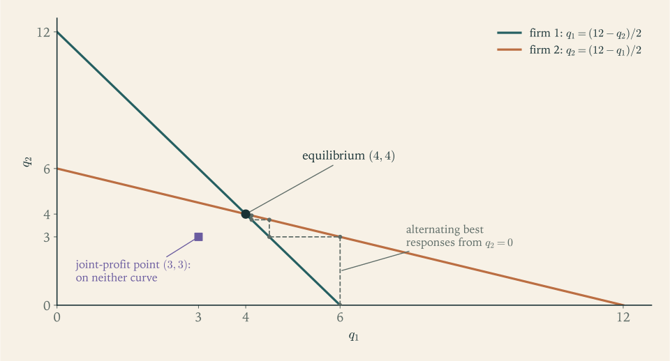
Figure 2.1 shows the two reaction lines and their crossing. It also shows a path of alternating best responses: starting from \(q_2=0\) , firm 1 replies with \(6\) , firm 2 replies to \(6\) with \(3\) , firm 1 replies to \(3\) with \(4.5\) , and so on. Because each reaction function has slope \(-1/2\) , every reply halves the distance to the equilibrium quantity, and the path converges to \((4,4)\) . This illustrates the rest-point reading of equilibrium. It is a property of this model, not of games in general: with other reaction functions the same process can cycle.

The same calculation handles \(n\) firms with a common cost \(c\) . Firm \(i\) ’s profit is \(q_i(a-c-q_i-Q_{-i})\) , where \(Q_{-i}\) is the output of the others, and the first-order condition is \(a-c-2q_i-Q_{-i}=0\) , that is, \(q_i=a-c-Q\) where \(Q\) is total output. The right-hand side is the same for every firm, so every equilibrium is symmetric, and \(q=a-c-nq\) gives

\[ q^\star=\frac{a-c}{n+1},\qquad Q^\star=\frac{n}{n+1}(a-c),\qquad P^\star=c+\frac{a-c}{n+1}. \]

With \(n=1\) this is the monopoly output, with \(n=2\) the duopoly output above, and as \(n\to\infty\) the price falls to the unit cost \(c\) .

2.5 Price competition

Now let the same two firms, with the common unit cost \(c\) , choose prices instead of quantities. Consumers buy only from the cheaper firm; total demand at price \(p\) is \(D(p)=a-p\) for \(p\le a\) and zero above; if the prices are equal the firms share the demand equally. Firm \(i\) ’s profit is \((p_i-c)D(p_i)\) if \(p_i<p_j\) , half of that if \(p_i=p_j\) , and \(0\) if \(p_i>p_j\) . This is the Bertrand duopoly. The payoff functions are discontinuous: an arbitrarily small price cut can double a firm’s sales. Calculus does not apply, and the equilibrium must be found by reasoning directly from Definition 2.1.

2.6 Many players

With many players a table is impossible and calculus may not apply either, but the definition can still be checked directly, often by counting.

Exercises

1. Find all pure Nash equilibria of \(\begin{array}{c|ccc}& L & C & R\\\hline T&(5,5)&(0,6)&(2,1)\\ M&(6,0)&(3,3)&(1,2)\\ B&(1,2)&(2,1)&(4,4)\end{array}\) by marking best responses, and for the cell \((T,L)\) name every player who has a profitable deviation and the deviation.

   Answer

   Player 1’s best responses are \(M\) to \(L\) , \(M\) to \(C\) , and \(B\) to \(R\) ; player 2’s are \(C\) to \(T\) , \(C\) to \(M\) , and \(R\) to \(B\) . The pure Nash equilibria are \((M,C)\) with payoffs \((3,3)\) and \((B,R)\) with payoffs \((4,4)\) . At \((T,L)\) both players have a profitable deviation: player 1 to \(M\) (from \(5\) to \(6\) ) and player 2 to \(C\) (from \(5\) to \(6\) ). The cell with the highest payoffs for both is not an equilibrium.

2. In the game \(\begin{array}{c|cc}& L & R\\\hline T&(x,3)&(1,1)\\ B&(2,0)&(3,x)\end{array}\) find, for each real number \(x\) , the set of pure Nash equilibria. Present the answer as a list of ranges of \(x\) .

   Solution

   Test each cell with the two inequalities of Definition 2.1.

   \((T,L)\) : player 1 needs \(x\ge 2\) (comparing with \(B\) in column \(L\) ) and player 2 needs \(3\ge 1\) (comparing with \(R\) in row \(T\) ), which always holds. So \((T,L)\) is an equilibrium exactly when \(x\ge 2\) .

   \((T,R)\) : player 1 needs \(1\ge 3\) , which is false. Never an equilibrium.

   \((B,L)\) : player 1 needs \(2\ge x\) and player 2 needs \(0\ge x\) . So \((B,L)\) is an equilibrium exactly when \(x\le 0\) .

   \((B,R)\) : player 1 needs \(3\ge 1\) , always true, and player 2 needs \(x\ge 0\) . So \((B,R)\) is an equilibrium exactly when \(x\ge 0\) .

   Collecting the cases: for \(x<0\) the only equilibrium is \((B,L)\) ; for \(x=0\) the equilibria are \((B,L)\) and \((B,R)\) ; for \(0<x<2\) the only equilibrium is \((B,R)\) ; for \(x\ge 2\) they are \((T,L)\) and \((B,R)\) . The boundary values \(x=0\) and \(x=2\) produce equilibria that are not strict, because one of the inequalities holds with equality there.

3. Prove directly from Definition 2.1, without using Theorem 2.3, that if every player has a strictly dominant strategy then the profile of dominant strategies is a Nash equilibrium and there is no other.

   Solution

   Let \(t_i\) be the strictly dominant strategy of player \(i\) and \(t=(t_1,\dots,t_n)\) . By definition \(u_i(t_i,s_{-i})>u_i(s_i,s_{-i})\) for every \(s_i\ne t_i\) and every \(s_{-i}\) . Taking \(s_{-i}=t_{-i}\) gives \(u_i(t_i,t_{-i})>u_i(s_i,t_{-i})\) for every \(s_i\ne t_i\) , which is the equilibrium inequality for player \(i\) , in its strict form. This holds for every player, so \(t\) is a (strict) Nash equilibrium.

   Now let \(s\) be any Nash equilibrium and suppose \(s_i\ne t_i\) for some player \(i\) . Taking the dominance inequality at the opponent profile \(s_{-i}\) gives \(u_i(t_i,s_{-i})>u_i(s_i,s_{-i})\) , so player \(i\) has a profitable unilateral deviation from \(s\) , contradicting the assumption that \(s\) is an equilibrium. Hence \(s_i=t_i\) for every \(i\) , that is, \(s=t\) .

4. Prove that a profile in which every player uses a weakly dominant strategy is a Nash equilibrium. Then verify that in Example 1.6 the profile \((T,L)\) is a Nash equilibrium in which player 1 uses a weakly dominated strategy, and list all pure Nash equilibria of that game.

   Hint

   A weakly dominant strategy satisfies \(u_i(t_i,s_{-i})\ge u_i(s_i,s_{-i})\) for every \(s_i\) and every \(s_{-i}\) ; specialise \(s_{-i}\) to the other players’ weakly dominant strategies. For Example 1.6 the best responses are \(\operatorname{BR}_1(L)=\{T,M\}\) , \(\operatorname{BR}_1(R)=\{M,B\}\) , \(\operatorname{BR}_2(T)=\{L\}\) , \(\operatorname{BR}_2(M)=\{L,R\}\) , \(\operatorname{BR}_2(B)=\{R\}\) , and you should find four pure equilibria: \((T,L)\) , \((M,L)\) , \((M,R)\) , \((B,R)\) .

5. A student writes: “In the stag hunt, (Hare, Hare) is not an equilibrium, because both hunters do better at (Stag, Stag).” Identify the comparison the student made, state the comparison the definition requires, and carry it out for both hunters.

   Hint

   The student compared (Hare, Hare) with (Stag, Stag), two cells that differ in both players’ strategies. The definition compares (Hare, Hare) with (Stag, Hare) for player 1 and with (Hare, Stag) for player 2. In each case the deviator’s payoff falls from \(2\) to \(0\) .

6. Solve the Cournot duopoly with \(a=20\) and \(c_1=c_2=2\) : give the reaction functions, the equilibrium quantities, the price, and each firm’s profit, and compare total profit with the monopoly profit.

   Answer

   \(\operatorname{BR}_i(q_j)=\max\{0,(18-q_j)/2\}\) ; \(q_1^\star=q_2^\star=6\) ; price \(8\) ; each firm’s profit is \(6\cdot 6=36\) , so \(72\) in total. A monopolist would produce \(9\) at price \(11\) for a profit of \(81\) .

7. For the Cournot model with \(n=3\) firms, \(a=14\) , and common cost \(c=2\) , derive firm 1’s reaction function in terms of \(q_2+q_3\) , prove that every equilibrium is symmetric, and find the equilibrium quantities, price, and profits. Then state the price in the \(n\) -firm model and its limit as \(n\to\infty\) .

   Solution

   Write \(Q_{-1}=q_2+q_3\) . If \(Q_{-1}<12\) , firm 1’s profit on the range where the price is positive is \(q_1(12-q_1-Q_{-1})\) , a concave quadratic with derivative \(12-2q_1-Q_{-1}\) , so

   \[ \operatorname{BR}_1(q_2,q_3)=\max\Bigl\{0,\ \frac{12-q_2-q_3}{2}\Bigr\}, \]

   and similarly for the other firms.

   Every equilibrium is symmetric. In an equilibrium some firm must be active, since if all outputs were zero any firm would gain by producing \(6\) . Let \(Q\) be total output. For an active firm \(i\) the first-order condition \(12-2q_i-(Q-q_i)=0\) gives \(q_i=12-Q\) . An inactive firm \(j\) would need \(12-Q_{-j}=12-Q\le 0\) , but then the active firms would have \(q_i=12-Q\le 0\) , a contradiction. So all three firms are active and each produces the same quantity \(12-Q\) .

   The equilibrium. With \(q_i=q\) for all \(i\) , \(q=12-3q\) gives \(q_1=q_2=q_3=3\) . Total output is \(9\) , the price is \(14-9=5\) , and each firm earns \(3\cdot(5-2)=9\) . As a check, against \(Q_{-1}=6\) firm 1’s profit is \(q_1(6-q_1)\) , maximized at \(q_1=3\) .

   Many firms. In the \(n\) -firm model the price is \(P^\star=c+(a-c)/(n+1)\) , here \(2+12/(n+1)\) , which decreases to the unit cost \(c\) as \(n\to\infty\) .

8. In the Cournot duopoly with \(a=14\) , \(c_1=2\) , and \(c_2=5\) , find the equilibrium quantities, the price, and both profits. For which values of \(c_2\) does firm 2 produce nothing in equilibrium?

   Answer

   \(q_1^\star=(14-4+5)/3=5\) and \(q_2^\star=(14-10+2)/3=2\) ; the price is \(7\) ; profits are \(5\cdot 5=25\) and \(2\cdot 2=4\) . Firm 2 produces nothing when \(c_2\ge 8\) .

9. In the Bertrand duopoly of Example 2.5, suppose prices must be whole numbers. Show that \((2,2)\) and \((3,3)\) are both Nash equilibria, that \((4,4)\) is not, and that no profile with \(p_1\ne p_2\) is an equilibrium.

   Solution

   With \(a=14\) and \(c=2\) , a firm that is the only seller at price \(p\) earns \((p-2)(14-p)\) .

   \((2,2)\) is an equilibrium. Both earn \(0\) . Raising the price loses all customers for a profit of \(0\) ; lowering it to \(1\) or \(0\) sells below cost. No deviation gains.

   \((3,3)\) is an equilibrium. At the common price \(3\) , each firm earns \(\tfrac12\cdot 1\cdot 11=5.5\) . Raising the price gives \(0\) . The only lower prices are \(2\) , \(1\) , and \(0\) , giving \(0\) or a loss. Undercutting is unprofitable because the smallest possible cut already reaches cost.

   \((4,4)\) is not. Each firm earns \(\tfrac12\cdot 2\cdot 10=10\) . Cutting to \(3\) captures the whole market for \(1\cdot 11=11>10\) .

   Unequal prices. Let \(p_i<p_j\) , so firm \(j\) sells nothing and earns \(0\) . If \(p_i<2\) , firm \(i\) is losing money and gains by moving to \(2\) . If \(p_i=2\) , firm \(i\) earns \(0\) and gains by moving to \(3\) , which earns \(11\) if \(p_j>3\) and \(5.5\) if \(p_j=3\) . If \(3\le p_i<14\) , firm \(j\) gains by matching \(p_i\) , which earns half of \((p_i-2)(14-p_i)>0\) . If \(p_i\ge 14\) there are no sales and firm \(j\) gains by charging \(8\) . So no profile with unequal prices is an equilibrium. Whole-number prices create a second equilibrium, one price step above cost, because the undercutting argument of Example 2.5 needs arbitrarily small cuts.

10. Two firms sell differentiated products at zero cost. Firm \(i\) sets a price \(p_i\ge 0\) and sells \(12-2p_i+p_j\) units. Find the reaction functions, the equilibrium prices and profits, and the common price that would maximize joint profit. In which direction do the reaction functions slope, and how does that differ from the Cournot model?

    Answer

    Firm \(i\) maximizes \(p_i(12-2p_i+p_j)\) , so \(\operatorname{BR}_i(p_j)=(12+p_j)/4\) . The equilibrium is \(p_1=p_2=4\) , with sales \(8\) and profit \(32\) each. A common price \(p\) gives each firm \(p(12-p)\) , maximized at \(p=6\) with profit \(36\) each. The reaction functions slope upward: a higher rival price calls for a higher own price. In the Cournot model they slope downward.

11. Two neighbours contribute \(g_1,g_2\ge 0\) to a shared garden and \(u_i(g_1,g_2)=2\sqrt{g_1+g_2}-g_i\) . Find all Nash equilibria, and compare the equilibrium level of \(g_1+g_2\) with the level that maximizes \(u_1+u_2\) .

    Solution

    Fix \(g_j\) and consider \(f(g_i)=2\sqrt{g_i+g_j}-g_i\) on \(g_i\ge 0\) . It is concave, with derivative \(1/\sqrt{g_i+g_j}-1\) . If \(g_j<1\) the derivative vanishes at \(g_i=1-g_j>0\) , which is therefore the maximizer. If \(g_j\ge 1\) the derivative is at most \(0\) for all \(g_i\ge 0\) and the maximizer is \(g_i=0\) . So \(\operatorname{BR}_i(g_j)=\max\{0,1-g_j\}\) : each neighbour tops the total up to \(1\) and contributes nothing if it is already there.

    A profile is an equilibrium when \(g_1=\max\{0,1-g_2\}\) and \(g_2=\max\{0,1-g_1\}\) . If \(g_2>1\) then \(g_1=0\) , and then \(g_2=1\) , a contradiction; similarly \(g_1>1\) is impossible. So both are at most \(1\) and the two conditions reduce to the single equation \(g_1+g_2=1\) . Every point of the segment \(\{(g_1,g_2):g_1,g_2\ge 0,\ g_1+g_2=1\}\) is an equilibrium: a continuum of equilibria, all with the same total and with every division of the burden.

    The sum of payoffs is \(4\sqrt G-G\) with \(G=g_1+g_2\) , whose derivative \(2/\sqrt G-1\) vanishes at \(G=4\) . So the efficient total is \(G=4\) , four times the equilibrium total, and the sum of payoffs is \(4\) there against \(3\) in equilibrium. Each neighbour weighs the cost of a contribution against their own benefit only, ignoring the equal benefit to the other.

12. Five villages are equally spaced along a road and numbered \(1\) to \(5\) ; each contains one customer. Two shops simultaneously choose a village to locate in. Each customer buys from the nearer shop, and a customer equally distant from both is shared half and half. A shop’s payoff is its number of customers. Find all pure Nash equilibria.

    Solution

    If both shops choose the same village they share all five customers, \(2.5\) each.

    \((3,3)\) is an equilibrium. Against a rival at \(3\) , moving to village \(2\) yields \(2\) customers (those at \(1\) and \(2\) ), moving to village \(1\) yields \(1.5\) (the customer at \(1\) and half of the customer at \(2\) , who is equally far from \(1\) and \(3\) ), and villages \(4\) and \(5\) are mirror images. All are below \(2.5\) .

    There is no other. In any equilibrium each shop gets at least \(2.5\) , since a shop can always copy the rival’s location. The payoffs sum to \(5\) , so each gets exactly \(2.5\) . Now suppose the rival is at a village \(b\ne 3\) . If \(b>3\) , locating at \(3\) wins the customers at \(1\) , \(2\) , and \(3\) , at least \(3\) customers; if \(b<3\) , locating at \(3\) wins those at \(3\) , \(4\) , and \(5\) . Either way the best response to \(b\ne 3\) earns at least \(3>2.5\) , which is incompatible with equilibrium. So in equilibrium each shop’s rival is at \(3\) . The unique pure Nash equilibrium is \((3,3)\) : both shops in the middle village.

13. A two-player game has common interests if \(u_1=u_2\) . Prove that in a finite game with common interests, any profile that maximizes the common payoff is a Nash equilibrium. Give a \(2\times 2\) example with common interests that has a second Nash equilibrium with a lower payoff.

    Solution

    Let \(u=u_1=u_2\) and let \(s=(s_1,s_2)\) maximize \(u\) over all profiles; a maximizer exists because the game is finite. For any deviation \(t_1\) of player 1, \(u_1(t_1,s_2)=u(t_1,s_2)\le u(s)=u_1(s)\) , because \(u(s)\) is the largest value \(u\) takes anywhere. The same argument applies to player 2. So no unilateral deviation is profitable and \(s\) is a Nash equilibrium. Notice that the argument uses much less than was given: \(s\) need only be at least as good as the profiles that differ from it in one coordinate.

    For the example, let both players get \(2\) at \((T,L)\) , \(1\) at \((B,R)\) , and \(0\) at the other two cells. Then \((T,L)\) maximizes the common payoff. But \((B,R)\) is also an equilibrium: a unilateral deviation from it leads to a cell with payoff \(0<1\) . Common interests remove conflict, not the coordination problem.

14. In Example 2.3, start from \(q_2=0\) and compute the first four alternating best responses. Show that the distance from the equilibrium quantity \(4\) halves at each step, and explain this from the slope of the reaction functions.

    Answer

    The replies are \(6\) , \(3\) , \(4.5\) , \(3.75\) , at distances \(2\) , \(1\) , \(0.5\) , \(0.25\) from \(4\) . Since \(\operatorname{BR}(q)-4=(12-q)/2-4=-(q-4)/2\) , each reply halves the distance and flips its sign.

15. A two-player game has \(\operatorname{BR}_1(L)=\{T,M\}\) , \(\operatorname{BR}_1(C)=\{B\}\) , \(\operatorname{BR}_1(R)=\{M\}\) and \(\operatorname{BR}_2(T)=\{C\}\) , \(\operatorname{BR}_2(M)=\{L,R\}\) , \(\operatorname{BR}_2(B)=\{R\}\) . Find all pure Nash equilibria from this information alone, say which of them could be strict, and explain why the best-response sets do not determine which profiles are Pareto efficient.

    Hint

    A cell is an equilibrium when the row is in \(\operatorname{BR}_1\) of the column and the column is in \(\operatorname{BR}_2\) of the row. Run through the nine cells; you should find \((M,L)\) and \((M,R)\) . An equilibrium is strict only if both best-response sets involved are singletons, and \(\operatorname{BR}_2(M)\) has two elements. Best-response sets record comparisons within a column for player 1 and within a row for player 2; Pareto comparisons need payoffs across arbitrary cells, which they do not contain.

16. Three players each choose \(A\) or \(B\) . A player who chooses \(A\) gets \(2\) if at least one other player also chooses \(A\) and \(0\) otherwise; a player who chooses \(B\) gets \(1\) . Find all pure Nash equilibria, treating the eight profiles by the number of players who choose \(A\) .

    Answer

    Three \(A\) : each gets \(2\) and would get \(1\) from \(B\) ; equilibrium. Two \(A\) : the player on \(B\) gets \(1\) and would get \(2\) from \(A\) ; not an equilibrium. One \(A\) : that player gets \(0\) and would get \(1\) from \(B\) ; not an equilibrium. No \(A\) : each gets \(1\) and would get \(0\) from \(A\) ; equilibrium. The pure Nash equilibria are \((A,A,A)\) and \((B,B,B)\) .

17. Use Theorem 2.3 and the result of Exercise 4 of Chapter 1Chapter 1 to show that the game \(\begin{array}{c|ccc}& L & C & R\\\hline T&(4,2)&(2,6)&(5,1)\\ M&(2,1)&(0,7)&(3,5)\\ B&(5,3)&(5,5)&(1,7)\end{array}\) has no pure Nash equilibrium, examining only four cells.

    Hint

    By Exercise 4 of Chapter 1Chapter 1, iterated elimination leaves the rows \(T,B\) and the columns \(C,R\) . By Theorem 2.3(a) the equilibria of the full game are those of this \(2\times 2\) game. Mark best responses in its four cells and observe that no cell has both.

18. A student solves Example 2.3 by maximizing total profit \((q_1+q_2)(12-q_1-q_2)\) and splitting the answer equally, reporting the equilibrium \((3,3)\) . Explain what problem the student solved, compute the gain to firm 1 from its best deviation at \((3,3)\) , and state the equations that an equilibrium must satisfy instead.

    Answer

    The student solved the problem of a single owner of both firms. At \((3,3)\) firm 1 earns \(18\) ; its best response to \(3\) is \(4.5\) , which earns \(20.25\) , a gain of \(2.25\) . An equilibrium must satisfy \(q_1=(12-q_2)/2\) and \(q_2=(12-q_1)/2\) , one optimality condition for each firm with the other’s quantity held fixed.