A worker can Work or Shirk, and an employer can Inspect or Trust. Working costs the worker effort worth \(2\) and produces output worth \(6\) to the employer. The wage is \(4\) , paid unless the worker is caught shirking, and an inspection costs the employer \(1\) . The payoffs, with the worker as player 1, are

If the employer inspects, the worker should work; if the worker works, the employer should trust; if the employer trusts, the worker should shirk; and if the worker shirks, the employer should inspect. The best responses chase each other around the table and no cell is a Nash equilibrium. Yet situations of this kind are everywhere, in tax audits, ticket inspections, penalty kicks, and patrols, and they do not look chaotic. What one observes is that inspections happen some of the time, at a rate that nobody on the other side can predict on a given day.

That observation is the clue. Any predictable pattern of inspection would be exploited. An employer who must not be predictable has to make the choice in a way that the worker cannot anticipate, and the cleanest way to do that is to let chance decide. This chapter enlarges each player’s set of options to include randomized choices, shows that the inspection game then has an equilibrium, and develops the technique that finds such equilibria. The technique rests on a single observation that sounds wrong on first hearing: in an equilibrium, a player who randomizes must be exactly indifferent among the strategies being randomized over, so that player’s probabilities are determined by the opponent’s payoffs and not by the player’s own.

3.1 Randomizing

If \(S_i\) has \(k\) elements, \(\Delta(S_i)\) is the set of vectors in \(\mathbb R^k\) with nonnegative coordinates summing to one. For \(k=2\) it is a segment, described by one number; for \(k=3\) it is a triangle. Mixed strategies of different players are assumed to be carried out by independent randomizing devices, so the probability that the pure profile \(s=(s_1,\dots,s_n)\) results from the mixed profile \(\sigma=(\sigma_1,\dots,\sigma_n)\) is the product \(\sigma_1(s_1)\cdots\sigma_n(s_n)\) .

Using the same letter \(u_i\) for the original payoff and for its expectation is harmless, because the two agree on pure profiles. In a two-player game with payoff matrices \(A\) for player 1 and \(B\) for player 2, if player 1’s mixed strategy is the vector \(x\) and player 2’s is the vector \(y\) , the expected payoffs are \(x^{\top}Ay\) and \(x^{\top}By\) .

Two assumptions have entered. The first is independence, already mentioned. The second concerns the meaning of the payoff numbers. Players are now assumed to rank lotteries over outcomes by expected payoff, so the numbers must be von Neumann–Morgenstern utilities; a strictly increasing transformation that is not affine changes the ranking of lotteries, and the mixed equilibria move with it. An exercise shows this happening.

The structural fact on which everything rests is that expected payoff is linear in each player’s own probabilities.

The lemma is an instance of the linearity of expectation: the expectation of a weighted average of random payoffs is the weighted average of their expectations, whether or not the payoffs are independent (math.probability-theory.expectation-linearity). Its consequence for strategy is that a mixed strategy can never earn more than the best pure strategy in it. A weighted average of numbers cannot exceed the largest of them.

3.2 The indifference principle

Part (a) says that to check whether a mixed profile is an equilibrium it is enough to check deviations to pure strategies; there are finitely many of those. Part (c) is the indifference principle. It converts the search for a mixed equilibrium into algebra: guess which strategies each player uses, write down equations saying that each player’s used strategies all earn the same, solve, and then check the inequalities for the unused strategies.

Look at whose payoffs appear in which equations. The equalities for player \(i\) involve player \(i\) ’s payoffs and the other players’ probabilities. So the opponents’ mixtures are what make player \(i\) indifferent, and player \(i\) ’s own mixture is determined by the requirement that the opponents be indifferent.

3.3 Best-response curves in the unit square

When each of two players has two pure strategies, a mixed profile is a point \((q,p)\) of the unit square, and each player’s best-response correspondence can be drawn in it. For the inspection game, Example 3.1 gives the worker’s correspondence: \(p=0\) for \(q<1/2\) , \(p=1\) for \(q>1/2\) , and every \(p\in[0,1]\) at \(q=1/2\) . Its graph is a step with a vertical riser. The employer’s correspondence is \(q=1\) for \(p<3/4\) , \(q=0\) for \(p>3/4\) , and every \(q\in[0,1]\) at \(p=3/4\) : a step with a horizontal tread. By Proposition 2.2 applied to the mixed extension, the equilibria are the points lying on both graphs.

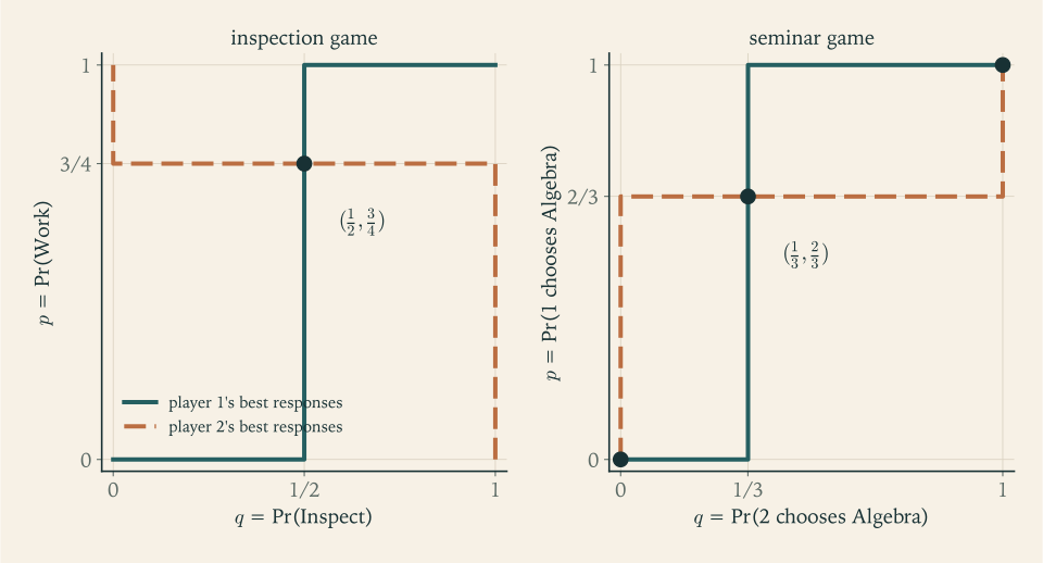
Figure 3.1 makes three things visible that the algebra hides. The graphs can cross only where at least one of them is on its flat segment or at a corner of the square, which is the indifference principle. In the left panel, following best responses from any corner of the square leads to the next corner and never stops, which is why no pure profile is stable. And the number of crossings is a property of how the two steps are oriented, which the next example illustrates.

3.4 Larger games: enumerating supports

With more than two strategies per player the picture is no longer available, but Theorem 3.4(c) still organizes the search. For each choice of a support for each player: write the equalities, add the conditions that the probabilities sum to one, solve the resulting linear system, discard solutions with negative probabilities, and check that no unused strategy earns more than the used ones. This is support enumeration. In a two-player game the equalities for player 1’s support are linear in player 2’s probabilities and conversely, so each step is linear algebra. For two players it is usually enough to try supports of equal size: if player 2 mixes over \(k\) strategies, there are \(k-1\) free probabilities with which to make player 1 indifferent among the strategies in player 1’s support, and for payoffs in general position that succeeds only when player 1’s support has at most \(k\) elements; by symmetry the two sizes are equal.

3.5 Dominance by a mixture

Mixed strategies also sharpen the tools of Chapter 1.

By Lemma 3.3 applied to the other players’ mixtures, the inequality then also holds against every mixed \(\sigma_{-i}\) , since \(u_i(\cdot,\sigma_{-i})\) is an average of the values \(u_i(\cdot,s_{-i})\) .

So strategies strictly dominated by mixtures may be deleted before looking for equilibria, and the deletion may be iterated as in Chapter 1. Theorem 2.3(a) remains true for this larger class of deletions, for mixed equilibria as well as pure ones, and its proof needs only one change: where a pure dominating strategy was compared with the dominated one against \(s_{-i}^\star\) , the dominating mixture is now compared with it against \(\sigma_{-i}^\star\) , whose support lies in the current reduction, and Theorem 3.4 turns the strict inequality into a contradiction with equilibrium. That is all the examples of this chapter use. Order independence, Theorem 1.7, is also true for iterated elimination by mixtures in finite games, but we quote it without proof. The chain argument of Chapter 1 does not transfer: a dominating mixture may put weight on strategies that are removed at the same step, the mixtures that dominate those may put weight back on the first, and so the process of replacing removed strategies by their dominators need not come to an end; a proof has to choose the dominating mixtures with more care. A related fact, which we state without proof because the proof belongs with the tools of Chapter 4, is that in a two-player game a pure strategy is strictly dominated by some mixed strategy if and only if it is not a best response to any mixed strategy of the opponent.

3.6 Many players, one symmetric mixture

The indifference principle is not confined to two players, though with three or more the equations are no longer linear, because the probability of each opponent profile is a product.

3.7 What a mixed equilibrium asserts

A mixed equilibrium has a peculiar feature: every player who randomizes is indifferent, so nobody has a strict incentive to use the equilibrium probabilities. Three interpretations make sense of this, and each is appropriate in some applications. A mixed strategy may be a deliberate randomization, adopted to prevent being outguessed, as by a goalkeeper or an auditor. It may describe a large population from which the players are drawn, in which a fraction \(\sigma_i(s_i)\) of the people in role \(i\) always play \(s_i\) ; the equilibrium condition then says that no type of behaviour does better than another. Or it may describe the beliefs of the other players about what player \(i\) will do, when player \(i\) in fact chooses on the basis of small private considerations that the others cannot observe; Chapter 7 makes this last reading precise.

Whatever the interpretation, the mathematics is the same, and two cautions apply. A mixed equilibrium is no less an equilibrium than a pure one: every pure equilibrium of \(G\) is an equilibrium of the mixed extension, by Theorem 3.4(a), and the mixed equilibria are additional solutions of the same definition. And enlarging the strategy sets has so far produced an equilibrium in every example. Whether it always does is a real question, with a real theorem as its answer, and it is the subject of Chapter 4.

Exercises

1. In the game \(\begin{array}{c|ccc}& L & C & R\\\hline T&(2,1)&(0,3)&(4,0)\\ B&(1,2)&(3,1)&(0,5)\end{array}\) let \(\sigma_1=(\tfrac13,\tfrac23)\) and \(\sigma_2=(\tfrac12,\tfrac14,\tfrac14)\) . Compute the expected payoff of each pure strategy of each player against the other’s mixture, both players’ expected payoffs from \((\sigma_1,\sigma_2)\) , and each player’s best responses to the other’s mixture.

   Answer

   Against \(\sigma_2\) : \(T\) earns \(2\cdot\tfrac12+0+4\cdot\tfrac14=2\) and \(B\) earns \(\tfrac12+\tfrac34+0=\tfrac54\) , so \(u_1(\sigma_1,\sigma_2)=\tfrac13\cdot 2+\tfrac23\cdot\tfrac54=\tfrac32\) and player 1’s only best response is \(T\) . Against \(\sigma_1\) : \(L\) earns \(\tfrac13+\tfrac43=\tfrac53\) , \(C\) earns \(1+\tfrac23=\tfrac53\) , and \(R\) earns \(\tfrac{10}{3}\) , so \(u_2(\sigma_1,\sigma_2)=\tfrac12\cdot\tfrac53+\tfrac14\cdot\tfrac53+\tfrac14\cdot\tfrac{10}{3}=\tfrac{25}{12}\) and player 2’s only best response is \(R\) .

2. Show that \(\begin{array}{c|cc}& L & R\\\hline T&(3,1)&(0,2)\\ B&(1,3)&(2,0)\end{array}\) has no pure equilibrium, find its mixed equilibrium by writing one labelled indifference equation for each player, and compute both equilibrium payoffs.

   Solution

   No pure equilibrium. Player 1’s best response to \(L\) is \(T\) (\(3>1\) ) and to \(R\) is \(B\) (\(2>0\) ). Player 2’s best response to \(T\) is \(R\) (\(2>1\) ) and to \(B\) is \(L\) (\(3>0\) ). No cell is a mutual best response.

   Let \(p\) be the probability of \(T\) and \(q\) the probability of \(L\) .

   Player 1 indifferent (determines \(q\) ). \(T\) earns \(3q\) and \(B\) earns \(q+2(1-q)=2-q\) . Setting \(3q=2-q\) gives \(q=1/2\) , and both earn \(3/2\) .

   Player 2 indifferent (determines \(p\) ). \(L\) earns \(p+3(1-p)=3-2p\) and \(R\) earns \(2p\) . Setting \(3-2p=2p\) gives \(p=3/4\) , and both earn \(3/2\) .

   Both players use both strategies, so there are no unused strategies to check. The equilibrium is \(\sigma_1=(\tfrac34,\tfrac14)\) and \(\sigma_2=(\tfrac12,\tfrac12)\) . Both equilibrium payoffs are \(3/2\) . Since against any pure strategy each player has a unique best response, no equilibrium has exactly one player mixing, so this is the only equilibrium.

3. Find all Nash equilibria, pure and mixed, of the stag hunt of Chapter 2. Explain the connection between the mixed equilibrium and the level of confidence \(p>2/3\) computed in Example 2.2.

   Answer

   The pure equilibria are (Stag, Stag) and (Hare, Hare). In the mixed equilibrium each hunter chooses Stag with probability \(2/3\) : the opponent’s probability \(p\) of Stag must make \(4p=3p+2(1-p)\) . The payoff is \(8/3\) each. This is the same equation as in Example 2.2: the mixed equilibrium sits exactly at the belief at which a hunter is indifferent, so \(2/3\) is the threshold separating the beliefs that lead to Stag from those that lead to Hare.

4. Prove that a strict Nash equilibrium of the mixed extension of a finite game is a profile of pure strategies.

   Hint

   Suppose \(\sigma_i^\star\) puts positive probability on two different pure strategies. By Theorem 3.4(c) both earn \(w_i\) against \(\sigma_{-i}^\star\) . So each of them, as a pure strategy, is a deviation from \(\sigma_i^\star\) that earns exactly as much as \(\sigma_i^\star\) , and it is different from \(\sigma_i^\star\) . What does strictness require of every deviation?

5. In the inspection game, suppose the cost of an inspection rises from \(1\) to \(2\) , so the employer’s payoffs in the Inspect column become \(0\) and \(-2\) . Find the new equilibrium and say which player’s behaviour changes, and why it is that player.

   Answer

   The employer is indifferent when \(2p-2=6p-4\) , so \(p^\star=1/2\) ; the worker’s condition is unchanged, so \(q^\star=1/2\) . The worker shirks more, half the time instead of a quarter, while the employer inspects exactly as often as before. The employer’s payoffs changed, and those payoffs determine the worker’s mixture.

6. A student solves the inspection game as follows: “The worker is indifferent when \(2p=4(1-p)\) , so \(p=2/3\) .” Identify what quantity the student’s equation should have contained, write the correct equation that determines \(p\) , and explain in one sentence why the worker’s own payoffs cannot determine \(p\) .

   Hint

   The student’s equation uses the worker’s payoffs \(2\) and \(4\) but weights them by the worker’s own probability. Lemma 3.3 says the worker’s two pure strategies earn \(2\) and \(4(1-q)\) , which involve \(q\) . The equation that determines \(p\) is the employer’s: \(2p-1=6p-4\) .

7. Find a Nash equilibrium of \(\begin{array}{c|ccc}& L & C & R\\\hline T&(2,6)&(4,1)&(3,0)\\ M&(4,2)&(0,5)&(2,6)\\ B&(5,1)&(1,1)&(1,6)\end{array}\) with supports \(\{T,M\}\) and \(\{L,R\}\) , verifying every condition of Theorem 3.4(c). Then show that the supports \(\{T,B\}\) and \(\{L,R\}\) do not give an equilibrium.

   Solution

   Supports \(\{T,M\}\) and \(\{L,R\}\) . Let player 2 play \(L\) with probability \(y\) and \(R\) with probability \(1-y\) . Then \(T\) earns \(2y+3(1-y)=3-y\) and \(M\) earns \(4y+2(1-y)=2+2y\) . Equality gives \(y=1/3\) and \(w_1=8/3\) . The unused strategy \(B\) earns \(5\cdot\tfrac13+1\cdot\tfrac23=\tfrac73\le\tfrac83\) .

   Let player 1 play \(T\) with probability \(x\) and \(M\) with probability \(1-x\) . Then \(L\) earns \(6x+2(1-x)=2+4x\) and \(R\) earns \(0\cdot x+6(1-x)=6-6x\) . Equality gives \(x=2/5\) and \(w_2=18/5\) . The unused strategy \(C\) earns \(1\cdot\tfrac25+5\cdot\tfrac35=\tfrac{17}{5}\le\tfrac{18}{5}\) .

   All probabilities are positive where they should be, the supported strategies earn equal payoffs, and the unsupported ones earn no more. By Theorem 3.4(c), \(\sigma_1=(\tfrac25,\tfrac35,0)\) and \(\sigma_2=(\tfrac13,0,\tfrac23)\) form a Nash equilibrium.

   Supports \(\{T,B\}\) and \(\{L,R\}\) . Player 1 is indifferent between \(T\) and \(B\) when \(3-y=5y+(1-y)=1+4y\) , that is, \(y=2/5\) , and then both earn \(2.6\) . But against \((\tfrac25,0,\tfrac35)\) the unused strategy \(M\) earns \(2+2\cdot\tfrac25=2.8\) . Since \(M\) earns \(2.8>2.6\) , the inequality for unused strategies fails and no equilibrium has these supports, whatever player 1’s probabilities are.

8. Player 1 has payoffs \((4,0)\) from \(T\) , \((0,4)\) from \(M\) , and \((1,2)\) from \(B\) against the columns \(L,R\) . Find every mixture \(aT+(1-a)M\) that strictly dominates \(B\) . Then verify directly that \(B\) is not a best response to any mixed strategy of player 2.

   Solution

   The mixture \(aT+(1-a)M\) earns \(4a\) against \(L\) and \(4(1-a)\) against \(R\) , while \(B\) earns \(1\) and \(2\) . Strict dominance requires \(4a>1\) and \(4(1-a)>2\) , that is, \(a>\tfrac14\) and \(a<\tfrac12\) . So the dominating mixtures are exactly those with \(\tfrac14<a<\tfrac12\) ; for example \(a=\tfrac38\) earns \((1.5,2.5)\) .

   For the direct verification, let player 2 play \(L\) with probability \(q\) . Then \(B\) earns \(q+2(1-q)=2-q\) , \(T\) earns \(4q\) , and \(M\) earns \(4-4q\) . If \(q\ge\tfrac12\) then \(T\) earns at least \(2\) , while \(B\) earns at most \(\tfrac32\) . If \(q\le\tfrac12\) then \(M\) earns at least \(2\) , while \(B\) earns \(2-q\) , which is less than \(2\) unless \(q=0\) , and at \(q=0\) the strategy \(M\) earns \(4\) . In every case some other strategy earns strictly more than \(B\) , so \(B\) is never a best response. This agrees with the fact quoted after Proposition 3.6: never a best response and strictly dominated by a mixture are the same thing in a two-player game.

9. In the volunteer’s dilemma with \(b=9\) and \(c=1\) , find the symmetric mixed equilibrium for \(n=2\) and for \(n=3\) , and the probability in each case that nobody volunteers. Then describe all pure equilibria for general \(n\) .

   Solution

   A volunteer gets \(b-c=8\) . A bystander who stays silent gets \(9\) times the probability that someone else volunteers. In a symmetric equilibrium with silence probability \(r\) , indifference requires \(8=9(1-r^{\,n-1})\) , so \(r^{\,n-1}=1/9\) .

   For \(n=2\) : \(r=1/9\) . Each person volunteers with probability \(8/9\) , and nobody volunteers with probability \(1/81\) .

   For \(n=3\) : \(r=(1/9)^{1/2}=1/3\) . Each person volunteers with probability \(2/3\) , and nobody volunteers with probability \(1/27\) . Adding a third bystander triples the chance that the report is never made.

   Pure equilibria. If exactly one person volunteers, that person gets \(8\) and would get \(0\) by staying silent, while each of the others gets \(9\) and would get \(8\) by volunteering too; nobody gains by deviating. If two or more volunteer, any one of them gains by staying silent (\(9>8\) ). If nobody volunteers, anyone gains by volunteering (\(8>0\) ). So the pure equilibria are exactly the \(n\) profiles with a single volunteer.

10. Prove that for any mixed profile \(\sigma_{-i}\) , the set of player \(i\) ’s mixed best responses to \(\sigma_{-i}\) is a convex subset of \(\Delta(S_i)\) : if \(\sigma_i\) and \(\sigma_i'\) are best responses, so is \(\lambda\sigma_i+(1-\lambda)\sigma_i'\) for every \(\lambda\in[0,1]\) .

    Hint

    Let \(w\) be the maximal pure payoff against \(\sigma_{-i}\) . By Theorem 3.4(b), a mixed strategy is a best response exactly when its support lies in the set \(M\) of pure strategies that earn \(w\) . The support of \(\lambda\sigma_i+(1-\lambda)\sigma_i'\) is contained in the union of the two supports. Alternatively, use Lemma 3.3 directly: the payoff of the combination is \(\lambda w+(1-\lambda)w\) .

11. In the seminar game, replace each of player 1’s payoffs \(u\) by \(u^3\) , leaving player 2’s payoffs alone. Find the mixed equilibrium of the new game and say which player’s probabilities changed. Then prove that replacing \(u_1\) by \(au_1+b\) with \(a>0\) changes no equilibrium, pure or mixed.

    Answer

    Player 1’s payoffs become \(8\) and \(1\) . Player 1 is indifferent when \(8q=1-q\) , so player 2 now chooses Algebra with probability \(q=1/9\) instead of \(1/3\) ; player 1’s probability \(p=2/3\) is unchanged, since player 2’s payoffs are unchanged. For the affine case, \(au_1(s_1,\sigma_2)+b\) is the expected value of \(au_1+b\) , and the comparisons in Theorem 3.4(c) are unaffected by multiplying by \(a>0\) and adding \(b\) .

12. Write the payoff table of rock–paper–scissors, with \(1\) for a win, \(-1\) for a loss, and \(0\) for a tie. Verify with Theorem 3.4(c) that both players mixing uniformly is an equilibrium, and show that there is no equilibrium in which some player uses exactly two of the three pure strategies.

    Hint

    For the uniform profile, every pure strategy earns \(\tfrac13(0+1-1)=0\) against the opponent’s mixture. For the second part, suppose player 1 uses only Rock and Paper, with probabilities \(x\) and \(1-x\) , both positive. Compute player 2’s three pure payoffs and show that Rock earns strictly less than Paper, so player 2 uses only Paper and Scissors. Then compute player 1’s payoffs against such a mixture and show that Scissors earns strictly more than Paper unless player 2’s mixture is impossible.

13. For the game \(\begin{array}{c|cc}& L & R\\\hline T&(1,1)&(0,0)\\ B&(1,0)&(2,1)\end{array}\) draw both best-response correspondences in the unit square, with \(q\) the probability of \(L\) and \(p\) the probability of \(T\) , and describe the full set of Nash equilibria.

    Solution

    Player 1. Against \(q\) , \(T\) earns \(q\) and \(B\) earns \(q+2(1-q)=2-q\) . So \(B\) is strictly better whenever \(q<1\) , and at \(q=1\) both earn \(1\) . Player 1’s correspondence is \(p=0\) for \(q<1\) and every \(p\in[0,1]\) at \(q=1\) : the bottom edge of the square together with its right edge.

    Player 2. Against \(p\) , \(L\) earns \(p\) and \(R\) earns \(1-p\) . So \(L\) is strictly better for \(p>\tfrac12\) , \(R\) for \(p<\tfrac12\) , and at \(p=\tfrac12\) every \(q\) is a best response. Player 2’s correspondence is the left edge up to \(p=\tfrac12\) , the horizontal segment at \(p=\tfrac12\) , and the right edge above \(p=\tfrac12\) .

    Crossings. On the bottom edge (\(p=0\) ) player 2 requires \(q=0\) : the point \((q,p)=(0,0)\) , which is the pure profile \((B,R)\) . On the right edge (\(q=1\) ) player 2 requires \(p\ge\tfrac12\) . So the set of Nash equilibria consists of \((B,R)\) together with the whole segment \(q=1\) and \(p\in[\tfrac12,1]\) : player 2 plays \(L\) and player 1 plays \(T\) with any probability of at least one half. This includes the pure equilibrium \((T,L)\) .

    The continuum arises because player 1 has a tie against \(L\) : the vertical part of player 1’s graph lies on the edge of the square and overlaps a vertical part of player 2’s graph. In all these equilibria player 1 uses \(T\) , which is weakly dominated by \(B\) .

14. Three firms simultaneously decide whether to enter a market. A firm that stays out gets \(0\) . An entrant gets \(4\) if it is the only entrant, \(0\) if there are exactly two entrants, and \(-1\) if all three enter. Find the symmetric mixed equilibrium and the probability that the market ends up with no entrant.

    Solution

    Let each firm enter with probability \(p\in(0,1)\) . From the point of view of one firm, the other two both stay out with probability \((1-p)^2\) , exactly one of them enters with probability \(2p(1-p)\) , and both enter with probability \(p^2\) . Entering therefore earns

    \[ 4(1-p)^2+0\cdot 2p(1-p)-p^2 , \]

    and staying out earns \(0\) . Indifference requires \(4(1-p)^2=p^2\) . Both sides are squares of nonnegative numbers, so \(2(1-p)=p\) and \(p=2/3\) .

    By Theorem 3.4(c), every firm entering with probability \(2/3\) is an equilibrium: each firm’s two pure strategies earn the same, \(0\) . The probability that no firm enters is \((1/3)^3=1/27\) , and the probability that all three enter and lose money is \((2/3)^3=8/27\) . The expected profit of every firm is zero, although a market worth \(4\) to a single entrant is available: the value is dissipated by the risk of crowding.

15. In the game \(\begin{array}{c|ccc}& L & C & R\\\hline T&(6,1)&(0,4)&(2,2)\\ M&(0,5)&(3,0)&(2,2)\\ B&(1,0)&(1,0)&(1,6)\end{array}\) carry out iterated elimination of strategies strictly dominated by mixtures, as in Chapter 1 but with Definition 3.5, and then find the unique Nash equilibrium.

    Answer

    \(B\) is strictly dominated by \(\tfrac12T+\tfrac12M\) , which earns \((3,1.5,2)\) against \((1,1,1)\) . With \(B\) gone, \(R\) earns \((2,2)\) against \((T,M)\) and is strictly dominated by \(\tfrac12L+\tfrac12C\) , which earns \((2.5,2.5)\) . In the remaining game, player 1 is indifferent when \(6y=3(1-y)\) , so \(L\) has probability \(1/3\) ; player 2 is indifferent when \(x+5(1-x)=4x\) , so \(T\) has probability \(5/8\) . The equilibrium is \(\sigma_1=(\tfrac58,\tfrac38,0)\) , \(\sigma_2=(\tfrac13,\tfrac23,0)\) with payoffs \((2,\tfrac52)\) .

16. In the hawk–dove game two animals contest a resource worth \(4\) . Two hawks fight and each gets \(-1\) ; a hawk takes everything from a dove; two doves share. The table is \(\begin{array}{c|cc}& H & D\\\hline H&(-1,-1)&(4,0)\\ D&(0,4)&(2,2)\end{array}\) . Find all equilibria and interpret the symmetric one as a statement about a population of animals.

    Answer

    Pure equilibria: \((H,D)\) and \((D,H)\) . Mixed: each plays \(H\) with probability \(2/3\) , from \(-q+4(1-q)=2(1-q)\) , with expected payoff \(2/3\) . Read as a population statement: when two thirds of the animals are hawks, hawks and doves do equally well, so neither kind of behaviour can spread at the expense of the other.

17. Prove that a \(2\times 2\) game with no pure Nash equilibrium has no ties in the relevant comparisons, that is, each player has a unique best response to each pure strategy of the other, and deduce that it has exactly one Nash equilibrium, in which both players mix over both strategies.

    Solution

    Call the rows \(T,B\) and the columns \(L,R\) .

    No ties. Suppose player 1 were indifferent between \(T\) and \(B\) against some column, say \(L\) . Then both \(T\) and \(B\) are best responses to \(L\) . Since \((T,L)\) is not an equilibrium, \(L\) is not a best response to \(T\) , so player 2 strictly prefers \(R\) against \(T\) . Since \((B,L)\) is not an equilibrium, player 2 strictly prefers \(R\) against \(B\) as well. Then \(R\) is a best response to both rows, and if \(r\) is any best response of player 1 to \(R\) , the profile \((r,R)\) is a pure equilibrium, a contradiction. The same argument with the roles exchanged excludes ties for player 2.

    The best responses cycle. So each player has a unique best response to each pure strategy. Player 1’s best responses to \(L\) and \(R\) must differ, since otherwise that row would be strictly dominant and its best reply would give a pure equilibrium; likewise player 2’s best responses to \(T\) and \(B\) differ.

    Uniqueness. Because player 1’s payoff difference between \(T\) and \(B\) is strictly positive against one column and strictly negative against the other, and it is linear in \(q\) , it vanishes at exactly one \(q^\star\in(0,1)\) . Similarly player 2 is indifferent at exactly one \(p^\star\in(0,1)\) . In an equilibrium neither player can use a pure strategy: the other would reply with the unique pure best response, to which the first player’s unique best response is again pure, giving a pure equilibrium. So both mix, and by Theorem 3.4(c) each must be indifferent, forcing \(q=q^\star\) and \(p=p^\star\) . Conversely \((p^\star,q^\star)\) satisfies Theorem 3.4(c). There is exactly one equilibrium.

18. Use Theorem 3.4(a) to prove that every pure Nash equilibrium of a finite game \(G\) is a Nash equilibrium of its mixed extension. Then explain why the Cournot game of Chapter 2 is not covered by the definitions of this chapter, and what in the argument for Lemma 3.3 would need to change to cover it.

    Hint

    If \(s^\star\) is a pure equilibrium, then \(u_i(s_i^\star,s_{-i}^\star)\) is the largest pure payoff against \(s_{-i}^\star\) , and Theorem 3.4(a) bounds every mixed deviation by that number. In the Cournot game the strategy sets are infinite, so a mixed strategy is a probability distribution on \([0,\infty)\) and the sums in Definition 3.2 and Lemma 3.3 become integrals.