Lebesgue explained his integral with a story about paying a debt. One can take coins and notes out of a pocket in whatever order they come and add up their values one at a time; or one can first sort them by denomination, count how many there are of each, and then multiply and add. Both procedures give the same total, but the second is indifferent to the order in which the money was found. Riemann’s integral is the first procedure: it walks along the domain, interval by interval, and so it depends on the function being well behaved along the domain. Lebesgue’s is the second: it asks, for each value, how large the set is on which that value is taken, and it is indifferent to how that set is arranged.

Figure 4.1 shows the two procedures for one function. On the left the domain is cut into eight strips and each strip contributes its width times the smallest value of the function on it. On the right the range is cut into slabs of height \(\tfrac14\) and the function is rounded down to the slab boundary; the contribution of a level is its height times the measure of the set where the rounded function has that height. That set is a union of two intervals for the upper levels, and for a wilder function it could be any measurable set at all.

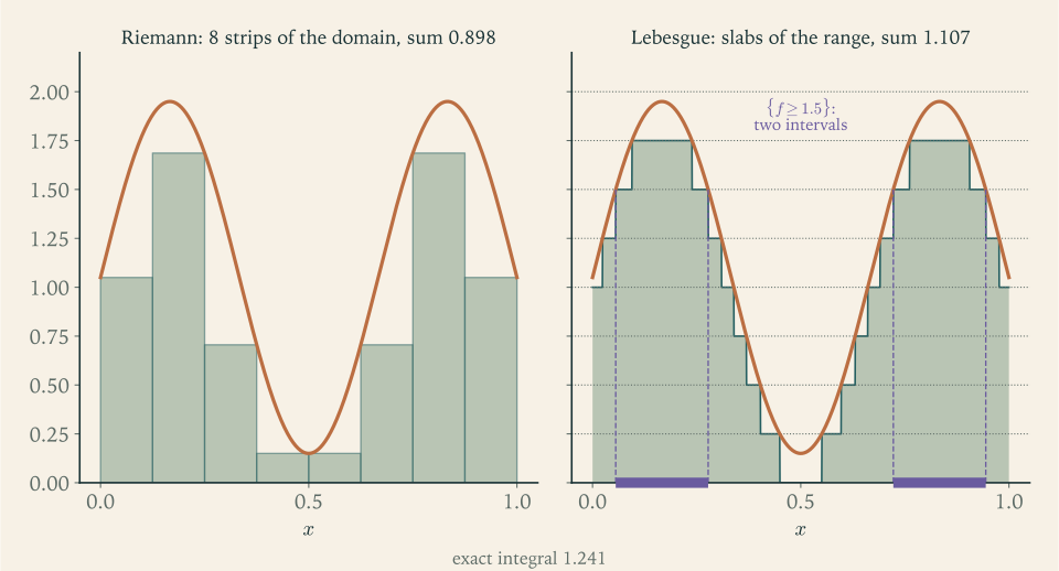
The plan is to define the integral in three steps: for nonnegative simple functions, where it is a finite sum; for nonnegative measurable functions, as a supremum; and for signed functions, by subtraction. The first limit theorem, on increasing sequences, is what holds the construction together: even the additivity of the integral is proved with it.

4.1 The integral of a simple function

Throughout, \((X,\mathcal A,\mu)\) is a measure space and all functions are measurable.

Part (a) is the coin-sorting principle: the total does not depend on how the money is grouped. Part (d) looks like a curiosity, and it is the key to the main theorem of the chapter.

4.2 Nonnegative measurable functions

When \(f\) is itself simple the supremum is attained at \(\varphi=f\) , by Lemma 4.2(c), so the two definitions agree. Two properties are immediate from the definition: if \(f\le g\) then \(\int f\,d\mu\le\int g\,d\mu\) , since the supremum for \(g\) is over a larger family; and \(\int cf\,d\mu=c\int f\,d\mu\) for \(c\ge0\) . One property is conspicuously not immediate. A simple function below \(f+g\) need not be a sum of a simple function below \(f\) and one below \(g\) , so the definition does not show that \(\int(f+g)\,d\mu=\int f\,d\mu+\int g\,d\mu\) . That will have to wait for the next section.

Other notations for the same number are \(\int_Xf\,d\mu\) and \(\int f(x)\,d\mu(x)\) , and for Lebesgue measure on an interval, \(\int_a^bf(x)\,dx\) . The last notation is the one used for the Riemann integral, and Section 4.5 proves that there is no conflict: for a continuous function on a compact interval the two integrals are the same number. The examples below use that fact, and with it the fundamental theorem of calculus, to evaluate integrals of continuous functions; no proof depends on it before it is established.

4.3 The monotone convergence theorem

The factor \(c<1\) is not decoration. With \(c=1\) the sets \(E_n\) need not exhaust \(X\) : if \(f_n=(1-\tfrac1n)\varphi\) , then \(f_n<\varphi\) wherever \(\varphi>0\) , for every \(n\) . The slack is what converts convergence at each point into membership in \(E_n\) from some index on. And the appeal to continuity from below, for the measure \(\nu\) , is the one place where countable additivity of \(\mu\) is used; the theorem is that continuity, transferred from sets to functions.

The hypotheses are three: measurable, nonnegative, increasing. Nothing is assumed about the size of the integrals. In particular the theorem can be used to prove that an integral is finite, or infinite, by computing the limit of the approximating integrals.

The first sentence of the proof also settles a practical point. To compute \(\int f\,d\mu\) one does not need the supremum over all simple functions below \(f\) ; any one increasing sequence of simple functions converging to \(f\) will do. For \(f(x)=3x\) on \([0,1]\) , Example 3.3 and Exercise 3.15 found the integrals \(\tfrac32-2^{-n-1}\) of the dyadic approximants, so \(\int_{[0,1]}3x\,d\lambda=\tfrac32\) .

The function \(f\) is called a density of \(\nu\) with respect to \(\mu\) . The second half of the proof is the three-stage method announced after Theorem 3.9, run in full for the first time. Chapter 9 asks the converse question: which measures \(\nu\) have a density with respect to a given \(\mu\) ?

Part (a) is Markov’s inequality, the simplest and most frequently used estimate in the subject. Part (d) says that the integral cannot see null sets. Consequently Theorems 4.4 and 4.5 remain true when their hypotheses hold only almost everywhere: redefine the functions to be \(0\) on the exceptional null set, which changes no integral.

4.4 Integrable functions

Since \(f^{\pm}\le\lvert f\rvert\) , both terms are finite and the difference makes sense. More generally the same formula defines \(\int f\,d\mu\in[-\infty,\infty]\) whenever at least one of \(\int f^+\,d\mu\) , \(\int f^-\,d\mu\) is finite; if both are infinite the integral is not defined. An integrable function is finite a.e. by Proposition 4.7(c), so sums of integrable functions are defined a.e., which is all that is needed.

One more property of a single integrable function will be needed in Chapters 9 and 10. It says that the mass of an integrable function cannot concentrate on small sets.

4.5 The Riemann integral as a special case

A bounded function \(f\) on \([a,b]\) is Riemann integrable when, for partitions \(P\) of \([a,b]\) , the upper sums \(U(f,P)\) and lower sums \(L(f,P)\) can be brought arbitrarily close together; the common limit is the Riemann integral (math.real-analysis.riemann-integrability).

The proof shows that a Riemann integrable function agrees almost everywhere with a Borel function, though it need not be Borel itself. Pushing the argument a little further yields Lebesgue’s characterization: a bounded function on \([a,b]\) is Riemann integrable exactly when its set of discontinuities has measure zero. So the Riemann integrable functions are the bounded functions that are continuous almost everywhere, a much narrower class than the bounded measurable functions.

For improper Riemann integrals the relationship is subtler. If the improper integral of \(\lvert f\rvert\) converges, the truncation argument of Example 4.3 shows that \(f\) is Lebesgue integrable with the same integral. If the improper integral converges only because of cancellation, the Lebesgue integral does not exist.

Exercises

1. Compute \(\int\varphi\,d\lambda\) for \(\varphi=2\cdot\mathbf 1_{[0,3]}+5\cdot\mathbf 1_{[1,2]}\) in two ways: from its standard representation, and directly from the given formula using linearity. Why does Lemma 4.2(a) not apply to the given formula?

   Answer

   The standard representation has value \(2\) on \([0,1)\cup(2,3]\) , of measure \(2\) , and value \(7\) on \([1,2]\) , of measure \(1\) , so the integral is \(2\cdot2+7\cdot1=11\) . By linearity, \(2\cdot3+5\cdot1=11\) . Lemma 4.2(a) requires pairwise disjoint sets, and \([0,3]\) and \([1,2]\) overlap; the given formula is handled by Lemma 4.2(b) instead.

2. On \(\mathbb N\) with counting measure, prove that \(\int f\,d\#=\sum_kf(k)\) for \(f\ge0\) , describe \(L^1(\#)\) , and restate Theorem 4.5 as a theorem about double series of nonnegative terms.

   Solution

   Let \(f:\mathbb N\to[0,\infty]\) . If \(f(k)=\infty\) for some \(k\) , then \(\infty\cdot\mathbf 1_{\{k\}}\) dominates simple functions \(c\mathbf 1_{\{k\}}\) of arbitrarily large integral \(c\) , and both sides are \(\infty\) . Otherwise the functions \(f_N=f\mathbf 1_{\{1,\dots,N\}}\) are simple, with \(\int f_N\,d\#=\sum_{k\le N}f(k)\) by Definition 4.1, since each singleton has counting measure \(1\) . They increase to \(f\) , so monotone convergence gives \(\int f\,d\#=\lim_N\sum_{k\le N}f(k)=\sum_kf(k)\) .

   A sequence \(f\) is integrable when \(\sum_k\lvert f(k)\rvert<\infty\) , so \(L^1(\#)\) is the space of absolutely summable sequences, and then \(\int f\,d\#=\sum_kf^+(k)-\sum_kf^-(k)=\sum_kf(k)\) .

   Theorem 4.5 with \(f_n(k)=a_{n,k}\ge0\) becomes: for any doubly indexed family of nonnegative numbers,

   \[ \sum_{k=1}^\infty\sum_{n=1}^\infty a_{n,k}=\sum_{n=1}^\infty\sum_{k=1}^\infty a_{n,k}, \]

   both sides possibly infinite. The order of summation of a nonnegative double series never matters.

3. Let \(f\) be the function on \([0,1]\) that vanishes on the Cantor set and equals \(n\) on each of the \(2^{n-1}\) open intervals removed at stage \(n\) of its construction. Compute \(\int f\,d\lambda\) .

   Solution

   Let \(G_n\) be the union of the \(2^{n-1}\) open intervals removed at stage \(n\) ; each has length \(3^{-n}\) , so \(\lambda(G_n)=2^{n-1}3^{-n}\) . The sets \(G_n\) are pairwise disjoint and \(f=\sum_{n\ge1}n\mathbf 1_{G_n}\) , a series of nonnegative measurable functions. By Theorem 4.5,

   \[ \int f\,d\lambda=\sum_{n=1}^\infty n\,2^{n-1}3^{-n}=\frac12\sum_{n=1}^\infty n\Bigl(\frac23\Bigr)^n . \]

   For \(\lvert r\rvert<1\) , \(\sum_{n\ge1}nr^n=\dfrac{r}{(1-r)^2}\) , and with \(r=\tfrac23\) this is \(\tfrac23\cdot9=6\) . Hence \(\int f\,d\lambda=3\) .

   The function is unbounded and it is discontinuous at every point of the Cantor set, but neither matters. The values on the Cantor set itself are irrelevant because that set is null. As a check on the bookkeeping, \(\sum_n\lambda(G_n)=\tfrac12\sum_n(\tfrac23)^n=1\) , so the removed intervals account for the whole length of \([0,1]\) .

4. Let \(f_n\) be measurable with \(f_1\ge f_2\ge\cdots\ge0\) and \(f_n\to f\) pointwise. Prove that \(\int f_n\,d\mu\to\int f\,d\mu\) provided \(\int f_1\,d\mu<\infty\) , and show by example that the proviso cannot be dropped.

   Solution

   Since \(f_1\ge f_n\ge0\) , the functions \(g_n=f_1-f_n\) are nonnegative wherever \(f_1<\infty\) , which is almost everywhere by Proposition 4.7(c) because \(\int f_1\,d\mu<\infty\) . They increase to \(f_1-f\) . By monotone convergence, in its almost-everywhere form,

   \[ \int(f_1-f_n)\,d\mu\longrightarrow\int(f_1-f)\,d\mu . \]

   All of \(f_1,f_n,f\) are integrable, being nonnegative and at most \(f_1\) . By linearity (Theorem 4.9) the left side is \(\int f_1\,d\mu-\int f_n\,d\mu\) and the right side is \(\int f_1\,d\mu-\int f\,d\mu\) . Subtracting the finite number \(\int f_1\,d\mu\) gives \(\int f_n\,d\mu\to\int f\,d\mu\) .

   The proviso is needed: \(f_n=\mathbf 1_{[n,\infty)}\) on \(\mathbb R\) decreases to \(0\) with \(\int f_n\,d\lambda=\infty\) for all \(n\) . It suffices that some \(f_m\) be integrable, since the sequence can be started at \(m\) . This is the function version of continuity from above, Theorem 1.10(b), and it has the same hypothesis for the same reason: a subtraction.

5. Let \(\mu(X)=1\) and let \(f\ge0\) have \(\int f\,d\mu=10\) . Give the best upper bound for \(\mu(\{f\ge50\})\) that follows from Markov’s inequality and exhibit a function on a two-point space for which it is attained.

   Answer

   \(\mu(\{f\ge50\})\le\tfrac{10}{50}=\tfrac15\) . Equality holds on \(X=\{a,b\}\) with \(\mu(\{a\})=\tfrac45\) , \(\mu(\{b\})=\tfrac15\) , \(f(a)=0\) , \(f(b)=50\) : then \(\int f\,d\mu=10\) and \(\mu(\{f\ge50\})=\tfrac15\) . Markov’s inequality is sharp exactly when \(f\) takes only the values \(0\) and \(t\) .

6. Let \(f\in L^1(\mu)\) . Prove that \(n\,\mu(\{\lvert f\rvert\ge n\})\to0\) as \(n\to\infty\) , which is stronger than what Markov’s inequality gives directly.

   Solution

   Let \(E_n=\{\lvert f\rvert\ge n\}\) . On \(E_n\) we have \(n\le\lvert f\rvert\) , so

   \[ n\,\mu(E_n)=\int n\mathbf 1_{E_n}\,d\mu\le\int\lvert f\rvert\mathbf 1_{E_n}\,d\mu . \]

   It remains to show that the right side tends to \(0\) . The functions \(\lvert f\rvert\mathbf 1_{E_n^c}=\lvert f\rvert\mathbf 1_{\{\lvert f\rvert<n\}}\) are nonnegative and increase with \(n\) , and they converge to \(\lvert f\rvert\) at every point where \(\lvert f\rvert<\infty\) , hence almost everywhere by Proposition 4.7(c). By monotone convergence \(\int\lvert f\rvert\mathbf 1_{E_n^c}\,d\mu\uparrow\int\lvert f\rvert\,d\mu\) , a finite number. Subtracting,

   \[ \int\lvert f\rvert\mathbf 1_{E_n}\,d\mu=\int\lvert f\rvert\,d\mu-\int\lvert f\rvert\mathbf 1_{E_n^c}\,d\mu\longrightarrow0 . \]

   Markov’s inequality alone gives only that \(n\mu(E_n)\) is bounded by \(\int\lvert f\rvert\,d\mu\) ; the improvement comes from integrating over the shrinking set \(E_n\) instead of the whole space.

7. Prove that \((1-\tfrac xn)^n\mathbf 1_{[0,n]}(x)\) increases with \(n\) for each \(x\ge0\) , and use monotone convergence to evaluate \(\lim_{n\to\infty}\int_0^n(1-\tfrac xn)^ne^{x/2}\,dx\) .

   Solution

   Monotonicity. Fix \(x\ge0\) and \(n\ge x\) . Apply the inequality between the geometric and arithmetic means to the \(n+1\) nonnegative numbers consisting of \(n\) copies of \(1-\tfrac xn\) and one copy of \(1\) :

   \[ \Bigl(1-\frac xn\Bigr)^{n/(n+1)}\le\frac{n(1-\tfrac xn)+1}{n+1}=1-\frac x{n+1}. \]

   Raising to the power \(n+1\) gives \((1-\tfrac xn)^n\le(1-\tfrac x{n+1})^{n+1}\) . For \(n<x\le n+1\) the left function is \(0\) by the indicator and the right one is nonnegative. So \(f_n(x)=(1-\tfrac xn)^ne^{x/2}\mathbf 1_{[0,n]}(x)\) is nonnegative and increasing in \(n\) , with limit \(e^{-x}e^{x/2}=e^{-x/2}\) .

   The limit. By monotone convergence,

   \[ \lim_{n\to\infty}\int_0^n\Bigl(1-\frac xn\Bigr)^ne^{x/2}\,dx=\int_0^\infty e^{-x/2}\,dx=2 , \]

   where the last integral is itself evaluated by monotone convergence from \(\int_0^Te^{-x/2}\,dx=2-2e^{-T/2}\) . For comparison, the first term of the sequence is \(\int_0^1(1-x)e^{x/2}\,dx=4\sqrt e-6\approx0.5949\) , so the convergence is slow.

8. A student reasons: “The functions \(\mathbf 1_{[n,n+1]}\) are nonnegative and converge to \(0\) everywhere, so by monotone convergence their integrals converge to \(0\) .” Each integral is \(1\) . State precisely which hypothesis fails.

   Answer

   The sequence is not increasing: \(\mathbf 1_{[1,2]}(1.5)=1>0=\mathbf 1_{[2,3]}(1.5)\) . Measurability and nonnegativity hold, and pointwise convergence holds, but monotone convergence requires \(f_n\le f_{n+1}\) . The mass slides off to infinity instead of accumulating.

9. Let \(K\) be the closed set of measure \(\tfrac12\) constructed in Example 2.5. Prove that \(\mathbf 1_K\) is not Riemann integrable on \([0,1]\) by bounding its upper and lower sums, and state its Lebesgue integral.

   Solution

   Let \(P\) be any partition of \([0,1]\) into subintervals \([x_{i-1},x_i]\) of positive length.

   Lower sums. The set \(K\) contains no interval, so each subinterval contains a point outside \(K\) , where \(\mathbf 1_K=0\) . The infimum of \(\mathbf 1_K\) on every subinterval is \(0\) and \(L(\mathbf 1_K,P)=0\) .

   Upper sums. On a subinterval that meets \(K\) the supremum is \(1\) ; on the others it is \(0\) . The subintervals that meet \(K\) cover \(K\) , so by monotonicity and subadditivity of \(\lambda\) their total length is at least \(\lambda(K)=\tfrac12\) . Hence \(U(\mathbf 1_K,P)\ge\tfrac12\) .

   Since \(U-L\ge\tfrac12\) for every partition, \(\mathbf 1_K\) is not Riemann integrable. It is a simple function, and its Lebesgue integral is \(\lambda(K)=\tfrac12\) .

   This agrees with Lebesgue’s criterion: \(\mathbf 1_K\) is discontinuous at every point of \(K\) , because every neighbourhood of such a point contains points outside \(K\) , and \(K\) has positive measure. For the ordinary Cantor set the same indicator is Riemann integrable, with integral \(0\) , because there the set of discontinuities is null.

10. Using truncations and monotone convergence, determine for which real \(p\) the function \(x^{-p}\) is Lebesgue integrable on \((0,1)\) , and for which \(p\) it is integrable on \((1,\infty)\) . Is it ever integrable on \((0,\infty)\) ?

    Answer

    On \((0,1)\) : integrable exactly when \(p<1\) , with integral \(\tfrac1{1-p}\) ; the truncated integrals over \([\tfrac1n,1]\) are \(\tfrac{1-n^{p-1}}{1-p}\) for \(p\ne1\) and \(\ln n\) for \(p=1\) . On \((1,\infty)\) : integrable exactly when \(p>1\) , with integral \(\tfrac1{p-1}\) . Never on \((0,\infty)\) , since no \(p\) satisfies both conditions.

11. Expand \(\dfrac{x}{e^x-1}\) as a series of nonnegative functions on \((0,\infty)\) and evaluate \(\int_0^\infty\dfrac{x}{e^x-1}\,dx\) , stating which theorem justifies integrating term by term.

    Solution

    For \(x>0\) we have \(0<e^{-x}<1\) , so the geometric series gives

    \[ \frac{x}{e^x-1}=\frac{xe^{-x}}{1-e^{-x}}=\sum_{k=1}^\infty xe^{-kx}, \]

    a series of nonnegative continuous functions on \((0,\infty)\) . Theorem 4.5 allows term-by-term integration of a series of nonnegative measurable functions with no further hypothesis. Each term is integrated by parts, on \([0,T]\) first and then letting \(T\to\infty\) by monotone convergence:

    \[ \int_0^\infty xe^{-kx}\,dx=\frac1{k^2}. \]

    Therefore

    \[ \int_0^\infty\frac{x}{e^x-1}\,dx=\sum_{k=1}^\infty\frac1{k^2}=\frac{\pi^2}6\approx1.6449 . \]

    The answer coincides with that of Example 4.4, which is no accident: the substitution \(x=-\ln(1-u)\) turns one integral into the other.

12. Let \(f\ge0\) be measurable and \(\nu(E)=\int_Ef\,d\mu\) . Prove that \(\mu(E)=0\) implies \(\nu(E)=0\) , and that if \(\mu\) is \(\sigma\) -finite and \(f<\infty\) a.e. then \(\nu\) is \(\sigma\) -finite.

    Hint

    If \(\mu(E)=0\) then \(f\mathbf 1_E=0\) a.e.; use Proposition 4.7(b). For \(\sigma\) -finiteness write \(X=\bigcup_nX_n\) with \(\mu(X_n)<\infty\) and consider the sets \(X_n\cap\{f\le m\}\) , on which \(\nu\) is at most \(m\mu(X_n)\) , together with the \(\nu\) -null set \(\{f=\infty\}\) .

13. Let \(f:\mathbb R\to[0,\infty]\) be Borel measurable, \(c>0\) , and \(t\in\mathbb R\) . Use Proposition 2.9 and the three-stage method to prove \(\int f(cx+t)\,d\lambda(x)=\frac1c\int f\,d\lambda\) .

    Solution

    Indicators. Let \(f=\mathbf 1_B\) with \(B\) a Borel set. Then \(f(cx+t)=1\) exactly when \(x\in c^{-1}(B-t)\) , a Borel set, being the preimage of \(B\) under the continuous map \(x\mapsto cx+t\) . By Proposition 2.9, first for the translation and then for the dilation by \(c^{-1}\) ,

    \[ \int\mathbf 1_B(cx+t)\,d\lambda(x)=\lambda\bigl(c^{-1}(B-t)\bigr)=\frac1c\lambda(B-t)=\frac1c\lambda(B)=\frac1c\int\mathbf 1_B\,d\lambda . \]

    Simple functions. Both sides of the identity are additive in \(f\) and homogeneous under multiplication by nonnegative constants, by Lemma 4.2(b). So it holds for nonnegative Borel simple functions.

    General \(f\) . Choose simple Borel \(\varphi_n\uparrow f\) by Theorem 3.9. Then \(\varphi_n(cx+t)\uparrow f(cx+t)\) for every \(x\) , and \(x\mapsto f(cx+t)\) is Borel measurable by Proposition 3.4. Apply monotone convergence to both sides of the identity for \(\varphi_n\) . For \(c<0\) the same proof gives the factor \(\tfrac1{\lvert c\rvert}\) .

14. Let \(f\in L^1(\lambda)\) on \(\mathbb R\) and \(F(x)=\int_{(-\infty,x]}f\,d\lambda\) . Use Proposition 4.10 to prove that \(F\) is uniformly continuous on \(\mathbb R\) .

    Hint

    For \(x<y\) , \(\lvert F(y)-F(x)\rvert\le\int_{(x,y]}\lvert f\rvert\,d\lambda\) . Given \(\varepsilon\) take the \(\delta\) of Proposition 4.10; the set \((x,y]\) has measure \(y-x\) , and the same \(\delta\) works for every \(x\) .

15. Find nonnegative measurable \(f_n\) on \(\mathbb R\) converging to \(0\) uniformly with \(\int f_n\,d\lambda=1\) for all \(n\) , and prove that on a space of finite measure uniform convergence of integrable functions does imply convergence of the integrals.

    Hint

    Try \(f_n=\tfrac1n\mathbf 1_{[0,n]}\) : the supremum is \(\tfrac1n\) and the integral is \(1\) . On a finite measure space, \(\lvert\int f_n\,d\mu-\int f\,d\mu\rvert\le\int\lvert f_n-f\rvert\,d\mu\le\mu(X)\sup\lvert f_n-f\rvert\) .

16. Let \(\varphi\) be a nonnegative simple function with positive values \(a_1<a_2<\dots<a_m\) , and put \(a_0=0\) . Prove the layer formula \(\int\varphi\,d\mu=\sum_{j=1}^m(a_j-a_{j-1})\,\mu(\{\varphi\ge a_j\})\) , and check it on the function of Exercise 4.1.

    Solution

    Let \(A_i=\{\varphi=a_i\}\) for \(i=1,\dots,m\) , so that \(\int\varphi\,d\mu=\sum_ia_i\mu(A_i)\) ; the set where \(\varphi=0\) contributes nothing. Because the values are ordered, \(\{\varphi\ge a_j\}=A_j\cup A_{j+1}\cup\dots\cup A_m\) , a disjoint union, so \(\mu(\{\varphi\ge a_j\})=\sum_{i\ge j}\mu(A_i)\) . Substitute and exchange the order of the two finite sums:

    \[ \sum_{j=1}^m(a_j-a_{j-1})\sum_{i=j}^m\mu(A_i)=\sum_{i=1}^m\mu(A_i)\sum_{j=1}^i(a_j-a_{j-1})=\sum_{i=1}^ma_i\,\mu(A_i), \]

    since the inner sum telescopes to \(a_i-a_0=a_i\) . If some \(\mu(A_i)\) is infinite both sides are infinite, as all terms are nonnegative.

    For the function of Exercise 4.1 the positive values are \(a_1=2\) and \(a_2=7\) , with \(\{\varphi\ge2\}=[0,3]\) and \(\{\varphi\ge7\}=[1,2]\) . The layer formula gives \((2-0)\cdot3+(7-2)\cdot1=11\) . This is the original expression \(2\cdot\mathbf 1_{[0,3]}+5\cdot\mathbf 1_{[1,2]}\) integrated term by term: writing a simple function as a stack of horizontal layers is the same as summing over nested sets, and it is the right-hand picture of Figure 4.1 read slab by slab.

17. For measurable \(f\ge0\) prove that \(\int f\,d\mu\) is the supremum, over all finite partitions of \(X\) into measurable sets \(A_1,\dots,A_m\) , of the lower sums \(\sum_j(\inf_{A_j}f)\,\mu(A_j)\) .

    Hint

    Pieces of measure zero contribute nothing and may be ignored. If \(\inf_{A_j}f=\infty\) on a piece of positive measure, then \(f=\infty\) there and both sides are infinite. Otherwise each lower sum is the integral of the simple function \(\sum_j(\inf_{A_j}f)\mathbf 1_{A_j}\le f\) , so the supremum is at most \(\int f\,d\mu\) . Conversely, a simple \(\varphi\le f\) with standard representation \(\sum a_j\mathbf 1_{A_j}\) satisfies \(a_j\le\inf_{A_j}f\) .