A walker stands on a hillside whose height above sea level at the map position \((x,y)\) is \(h(x,y)\) . She can set off in any compass direction. In which direction is the climb steepest, how steep is it, and in which directions could she walk without gaining or losing height at all?

A function of one variable has one slope at each point. A function of two variables has a slope for every direction, infinitely many numbers at a single point. The discovery of this chapter is that, for a well-behaved function, all of those slopes are encoded in one vector, the gradient, and are recovered from it by a dot product. The words “well-behaved” hide a real subtlety, and we shall see functions that have a slope in every direction and still fail to be well-behaved. Getting the definition right is the main work.

2.1 Functions of several variables and their level sets

A real-valued function of \(n\) variables assigns a number \(f(\mathbf x)\) to each point \(\mathbf x\) of a domain \(D\subseteq\mathbb R^n\) . For \(n=2\) there are two standard pictures. The graph is the surface \(z=f(x,y)\) in \(\mathbb R^3\) . The level set at height \(c\) is the set of points of the domain where \(f(x,y)=c\) ; for two variables it is usually a curve, and a drawing of several level curves is a contour map. A contour map is what the walker carries. Where contours crowd together the function changes quickly; along a contour it does not change at all.

For \(n=3\) the graph would live in four dimensions and cannot be drawn, so level sets carry the whole burden. The level sets of \(F(x,y,z)=x^{2}+y^{2}+z^{2}\) are spheres; a surface in space is very often presented as a level set \(F(x,y,z)=c\) and not as a graph. We keep both descriptions available, and Section 2.6 shows how the gradient treats them uniformly.

Throughout, a point \(\mathbf a\) is an interior point of \(D\) if some open ball \(\{\mathbf x:\lVert\mathbf x-\mathbf a\rVert<r\}\) with \(r>0\) is contained in \(D\) , and \(D\) is open if all its points are interior. Derivatives are defined at interior points, where the function can be compared with its values in every direction.

2.2 Limits and continuity

The definition is word for word the one-variable definition with absolute values replaced by norms, and the theory of sums, products, quotients, and compositions of continuous functions carries over unchanged; its development belongs to Real Analysis. In practice this means that any formula built from polynomials, roots, exponentials, logarithms, and trigonometric functions is continuous wherever it is defined. All the interest lies at exceptional points, typically where a denominator vanishes.

What is new in several variables is the phrase “whenever \(\lVert\mathbf x-\mathbf a\rVert<\delta\) ”. On the line a point can be approached from two sides. In the plane it can be approached along any line, any parabola, any spiral, and the definition demands the same limit along all of them at once. This gives a simple way to show that a limit does not exist: find two paths with different limits. It gives no way to show that a limit does exist; for that one needs an inequality valid in a whole neighbourhood.

2.3 Partial derivatives

The simplest way to differentiate a function of several variables is to freeze all the variables but one.

Geometrically, \(f_x(a,b)\) is the slope at \(x=a\) of the curve in which the graph meets the vertical plane \(y=b\) . Computationally it is an ordinary derivative in which the other variables are treated as constants, so every rule of single-variable calculus applies.

2.4 Differentiability and the tangent plane

The right generalization of the derivative is not a collection of slopes. It is the property that made the derivative useful in the first place: near the point, the function is well approximated by a linear one. In one variable, \(f\) is differentiable at \(a\) with derivative \(m\) exactly when \(f(a+h)=f(a)+mh+(\text{an error that is small compared with }h)\) , the local linear model of single-variable calculus (math.calculus.linearization-as-local-model). The same sentence makes sense in \(\mathbb R^n\) once \(mh\) is replaced by a dot product.

The numerator is the error made by the linear prediction \(f(\mathbf a)+\mathbf m\cdot\mathbf h\) . The definition requires that error to be small not merely in absolute terms but relative to the size of the step, uniformly over all directions of \(\mathbf h\) . That uniformity is what partial derivatives lack.

By Proposition 2.4, the gradient is the only candidate for the vector \(\mathbf m\) . So checking differentiability comes down to computing the partial derivatives and then deciding whether the linear prediction built from them has a relatively small error. Doing that from the definition each time would be tedious. Fortunately there is a criterion that covers nearly every function met in practice.

2.5 Directional derivatives and the gradient

Because \(\lVert\mathbf u\rVert=1\) , the point \(\mathbf a+t\mathbf u\) is at distance \(\lvert t\rvert\) from \(\mathbf a\) , so \(D_{\mathbf u}f(\mathbf a)\) is a rate of change per unit distance: the slope the walker experiences when she sets off in the direction \(\mathbf u\) . The partial derivatives are the directional derivatives in the coordinate directions.

The theorem turns infinitely many limits into one dot product. It also answers the walker’s questions at a stroke.

So the gradient is not just a list of partial derivatives. It is a geometric object: it points in the direction of fastest increase, and its length is the rate of that increase.

Example 2.5: Reading a hillside

Let the height be \(h(x,y)=100-x^{2}-2y^{2}\) , with \(x\) pointing east and \(y\) north, and let the walker stand at \((3,2)\) , at height \(h=83\) . The partial derivatives \(h_x=-2x\) and \(h_y=-4y\) are continuous, so \(h\) is differentiable and \(\nabla h(3,2)=(-6,-8)\) , a vector of length \(10\) .

By Corollary 2.9 the steepest climb is in the direction \((-\tfrac35,-\tfrac45)\) , roughly south-west and toward the summit at the origin but not straight at it, and the slope in that direction is \(10\) . If instead she walks north-east, \(\mathbf u=(1,1)/\sqrt2\) , the slope is

\[ D_{\mathbf u}h(3,2)=(-6,-8)\cdot\frac{(1,1)}{\sqrt2}=-7\sqrt2\approx-9.90 , \]

a steep descent. The level directions are the unit vectors orthogonal to the gradient, \(\pm(\tfrac45,-\tfrac35)\) ; setting off along either, she neither climbs nor descends to first order.

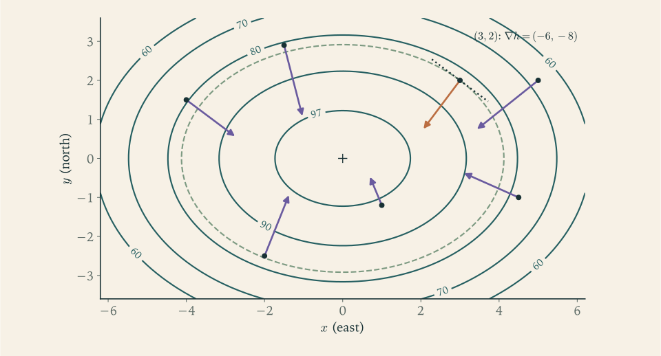
Figure 2.1 shows three things that the formula \(D_{\mathbf u}h=\nabla h\cdot\mathbf u\) states but does not display. Every arrow is perpendicular to the contour through its tail. The arrows are long near the rim, where the contours are packed, and short near the summit. And because the contours are ellipses and not circles, the arrows do not point at the summit: the direction of steepest ascent is a local matter, decided by the contour underfoot.

Common mistake. Using a direction vector that is not a unit vector. For \(f(x,y)=x+y\) the gradient is \((1,1)\) , and “the slope in the direction \((3,4)\) ” computed as \((1,1)\cdot(3,4)=7\) is too large by a factor of \(5\) , the length of \((3,4)\) . The slope per unit distance is \((1,1)\cdot(\tfrac35,\tfrac45)=\tfrac75\) . The number \(7\) is not meaningless: it is the rate of change of \(f\) per unit time for a point moving with velocity \((3,4)\) , as the next section shows. Decide which of the two you are being asked for, and normalize the direction when the question is about slope.

2.6 The gradient is perpendicular to level sets

The perpendicularity visible in Figure 2.1 is a theorem, and its proof introduces the first version of the multivariable chain rule: the derivative of a function along a moving point.

In coordinates, for \(z=f(x,y)\) with \(x=x(t)\) and \(y=y(t)\) , the theorem reads

each variable contributes its own rate of change times the sensitivity of \(f\) to that variable, and the contributions add. Taking \(\mathbf r(t)=\mathbf a+t\mathbf v\) shows that \(\nabla f(\mathbf a)\cdot\mathbf v\) is the rate of change of \(f\) per unit time for a point passing through \(\mathbf a\) with velocity \(\mathbf v\) , which settles the meaning of the number \(7\) in the last Common mistake.

This justifies a definition. If \(F\) is differentiable at a point \(\mathbf a\) of the level surface \(F(x,y,z)=c\) and \(\nabla F(\mathbf a)\ne\mathbf 0\) , the tangent plane to the surface at \(\mathbf a\) is the plane through \(\mathbf a\) with normal vector \(\nabla F(\mathbf a)\) :

A graph \(z=f(x,y)\) is the level surface \(F=0\) of \(F(x,y,z)=f(x,y)-z\) , whose gradient is \((f_x,f_y,-1)\) . The plane with that normal through \((a,b,f(a,b))\) is \(f_x(x-a)+f_y(y-b)-(z-f(a,b))=0\) , which is the tangent plane of Definition 2.5. The two definitions agree where both apply.

Exercises

1. State the definitions of a partial derivative, a directional derivative, and the gradient; say which of the three is a vector, which requires a unit vector in its definition, and which can exist at a point where the function is not continuous.

2. Describe the level curves \(f=c\) of \(f(x,y)=x^{2}-y^{2}\) for \(c=-1,0,1\) and the level surfaces \(F=c\) of \(F(x,y,z)=x^{2}+y^{2}-z^{2}\) for the same three values, naming each curve or surface.

   Answer

   Curves: \(x^{2}-y^{2}=1\) is a hyperbola opening left and right; \(x^{2}-y^{2}=0\) is the pair of lines \(y=\pm x\) ; \(x^{2}-y^{2}=-1\) is a hyperbola opening up and down. Surfaces: \(x^{2}+y^{2}-z^{2}=1\) is a hyperboloid of one sheet; \(x^{2}+y^{2}-z^{2}=0\) is a double cone with vertex at the origin; \(x^{2}+y^{2}-z^{2}=-1\) is a hyperboloid of two sheets.

3. Decide whether each limit at the origin exists, proving your answer with a pair of paths or with an inequality: (a) \(\dfrac{x^{2}-y^{2}}{x^{2}+y^{2}}\) ; (b) \(\dfrac{x^{3}+y^{3}}{x^{2}+y^{2}}\) ; (c) \(\dfrac{x^{2}y}{x^{4}+y^{2}}\) .

   Solution

   (a) Along the \(x\) -axis the quotient is \(x^{2}/x^{2}=1\) ; along the \(y\) -axis it is \(-y^{2}/y^{2}=-1\) . Two paths give different limits, so the limit does not exist.

   (b) For any point other than the origin, \(\lvert x\rvert^{3}=\lvert x\rvert\,x^{2}\le\lvert x\rvert(x^{2}+y^{2})\) and similarly \(\lvert y\rvert^{3}\le\lvert y\rvert(x^{2}+y^{2})\) . Hence

   \[ \Bigl\lvert\frac{x^{3}+y^{3}}{x^{2}+y^{2}}\Bigr\rvert\le\lvert x\rvert+\lvert y\rvert\le 2\lVert(x,y)\rVert . \]

   Given \(\varepsilon>0\) , take \(\delta=\varepsilon/2\) in Definition 2.1. So the limit is \(0\) .

   (c) Along a line \(y=mx\) with \(m\ne 0\) the quotient is \(mx^{3}/(x^{4}+m^{2}x^{2})=mx/(x^{2}+m^{2})\) , which tends to \(0\) ; along either axis it is identically \(0\) . But along the parabola \(y=x^{2}\) the quotient equals \(\tfrac12\) at every point, since \(x^{2}\cdot x^{2}/(x^{4}+x^{4})=\tfrac12\) . The line paths and the parabola disagree, so the limit does not exist. As in Example 2.1, agreement along all straight lines proves nothing.

4. Compute all first-order partial derivatives of (a) \(f(x,y)=x^{2}y^{3}+e^{xy}\) ; (b) \(g(x,y,z)=z\ln(x^{2}+y^{2})\) ; (c) \(h(x,y)=\arctan(y/x)\) , simplifying the last as far as possible.

   Answer

   (a) \(f_x=2xy^{3}+ye^{xy}\) , \(f_y=3x^{2}y^{2}+xe^{xy}\) . (b) \(g_x=2xz/(x^{2}+y^{2})\) , \(g_y=2yz/(x^{2}+y^{2})\) , \(g_z=\ln(x^{2}+y^{2})\) . (c) \(h_x=-y/(x^{2}+y^{2})\) , \(h_y=x/(x^{2}+y^{2})\) .

5. Find the tangent plane to the graph of \(f(x,y)=x^{2}y+y^{3}\) at \((1,2)\) , use it to estimate \(f(1.1,1.9)\) , and compare the estimate with the exact value.

   Solution

   The partial derivatives are \(f_x=2xy\) and \(f_y=x^{2}+3y^{2}\) , both continuous, so \(f\) is differentiable by Theorem 2.6. At \((1,2)\) : \(f=2+8=10\) , \(f_x=4\) , \(f_y=1+12=13\) . The tangent plane is \(z=10+4(x-1)+13(y-2)\) .

   The displacement to \((1.1,1.9)\) is \((0.1,-0.1)\) , so the linear estimate is \(10+0.4-1.3\) , that is, \(9.1\) . The exact value is \(1.21\cdot 1.9+1.9^{3}=2.299+6.859\) , that is, \(9.158\) . The error of the estimate is \(0.058\) , compared with a step of length \(\sqrt{0.02}\approx 0.14\) . The error is noticeably smaller than the step but not negligible, because the step is not very small and the second derivatives of \(f\) near \((1,2)\) are large; halving the step would roughly quarter the error.

6. Prove directly from Definition 2.3, without using Theorem 2.6, that \(f(x,y)=xy\) is differentiable at every point \((a,b)\) .

   Solution

   The candidate vector is the gradient, \(\nabla f(a,b)=(b,a)\) . For a displacement \(\mathbf h=(h,k)\) the error of the linear prediction is

   \[ f(a+h,b+k)-f(a,b)-bh-ak=(a+h)(b+k)-ab-bh-ak=hk . \]

   We must show that \(hk/\lVert\mathbf h\rVert\to 0\) . Since \((\lvert h\rvert-\lvert k\rvert)^{2}\ge 0\) , we have \(\lvert hk\rvert\le\tfrac12(h^{2}+k^{2})=\tfrac12\lVert\mathbf h\rVert^{2}\) . Therefore

   \[ \frac{\lvert hk\rvert}{\lVert\mathbf h\rVert}\le\tfrac12\lVert\mathbf h\rVert , \]

   which tends to \(0\) as \(\mathbf h\to\mathbf 0\) . Definition 2.3 holds with \(\mathbf m=(b,a)\) , so \(f\) is differentiable at \((a,b)\) . The error term \(hk\) is exactly the second-order part of the product, which is why the linearization of a product keeps only the terms in which one factor at a time is varied.

7. Show that \(f(x,y)=\sqrt{\lvert xy\rvert}\) has both partial derivatives equal to \(0\) at the origin, and prove that \(f\) is nevertheless not differentiable there.

   Solution

   On the \(x\) -axis \(f(t,0)=\sqrt{\lvert t\cdot 0\rvert}=0\) for every \(t\) , so the difference quotient \((f(t,0)-f(0,0))/t\) is identically \(0\) and \(f_x(0,0)=0\) . By symmetry \(f_y(0,0)=0\) .

   Suppose \(f\) were differentiable at the origin. By Proposition 2.4 the vector \(\mathbf m\) would be the gradient \((0,0)\) , so the quotient in Definition 2.3 would be \(f(\mathbf h)/\lVert\mathbf h\rVert\) , and it would have to tend to \(0\) as \(\mathbf h\to\mathbf 0\) along every path. Along the diagonal \(\mathbf h=(t,t)\) with \(t>0\) , however,

   \[ \frac{f(t,t)}{\lVert(t,t)\rVert}=\frac{\sqrt{t^{2}}}{\sqrt2\,t}=\frac1{\sqrt2} , \]

   which does not tend to \(0\) . So \(f\) is not differentiable at the origin. Geometrically the graph contains both coordinate axes, which would force a tangent plane to be horizontal, but along the diagonal the graph rises like the cone \(z=\lvert t\rvert\) , with a corner.

8. For \(f(x,y,z)=xy+yz^{2}\) and \(P=(1,2,-1)\) , compute the directional derivative of \(f\) at \(P\) in the direction from \(P\) toward \(Q=(3,1,1)\) , and find the largest directional derivative at \(P\) .

   Solution

   The partial derivatives are \(f_x=y\) , \(f_y=x+z^{2}\) , \(f_z=2yz\) ; they are continuous, so \(f\) is differentiable and Theorem 2.8 applies. At \(P=(1,2,-1)\) we get \(\nabla f(P)=(2,2,-4)\) .

   The direction from \(P\) to \(Q\) is \(Q-P=(2,-1,2)\) , of length \(3\) , so the unit vector is \(\mathbf u=\tfrac13(2,-1,2)\) . Then

   \[ D_{\mathbf u}f(P)=\tfrac13\,(2,2,-4)\cdot(2,-1,2)=\tfrac13(4-2-8)=-2 . \]

   The function decreases at \(2\) units per unit distance in that direction. By Corollary 2.9 the largest directional derivative at \(P\) is \(\lVert\nabla f(P)\rVert=\sqrt{4+4+16}=\sqrt{24}\) , that is, \(2\sqrt6\) , attained in the direction \((1,1,-2)/\sqrt6\) .

9. The temperature on a plate is \(T(x,y)=100/(1+x^{2}+2y^{2})\) . At the point \((1,1)\) , in which direction does the temperature fall fastest, and at what rate per unit distance?

   Answer

   \(\nabla T(1,1)=(-12.5,-25)\) . The temperature falls fastest in the direction of \(-\nabla T\) , the unit vector \((1,2)/\sqrt5\) , at the rate \(\lVert\nabla T(1,1)\rVert=12.5\sqrt5\approx 27.95\) degrees per unit distance.

10. A student asked for the slope of \(f(x,y)=x^{2}+y^{2}\) at \((1,1)\) in the direction of \(\mathbf v=(1,2)\) computes \(\nabla f(1,1)\cdot\mathbf v=6\) . Explain what is wrong with this answer as a slope, give the correct slope, and say what the number \(6\) does measure.

    Solution

    The gradient is \(\nabla f=(2x,2y)\) , which at \((1,1)\) is \((2,2)\) , and the student’s dot product \((2,2)\cdot(1,2)=6\) is computed correctly. The error is that Definition 2.7 and Theorem 2.8 require a unit vector, and \(\mathbf v=(1,2)\) has length \(\sqrt5\) . A slope is a change in height per unit of horizontal distance, and moving by \(t\mathbf v\) covers a distance of \(\sqrt5\,t\) , not \(t\) .

    The correct slope uses \(\mathbf u=\mathbf v/\sqrt5\) : it is \(6/\sqrt5\approx 2.68\) . The number \(6\) is still meaningful. By Theorem 2.10 applied to \(\mathbf r(t)=(1,1)+t\mathbf v\) , it is the rate of change of \(f\) per unit time for a point passing through \((1,1)\) with velocity \((1,2)\) . That point has speed \(\sqrt5\) , and dividing the time rate \(6\) by the speed returns the slope \(6/\sqrt5\) .

11. Prove that \(\nabla(fg)=f\,\nabla g+g\,\nabla f\) for differentiable \(f\) and \(g\) , and show that for \(\mathbf x\ne\mathbf 0\) the function \(\rho(\mathbf x)=\lVert\mathbf x\rVert\) has gradient \(\mathbf x/\lVert\mathbf x\rVert\) .

    Hint

    For the product rule, apply the single-variable product rule to each partial derivative. For the norm, write \(\rho=(x_1^{2}+\dots+x_n^{2})^{1/2}\) and differentiate with respect to \(x_i\) to get \(x_i/\rho\) . Then interpret: the distance from the origin increases fastest directly away from the origin, at rate \(1\) .

12. Find the tangent plane and the normal line to the surface \(xyz=6\) at the point \((1,2,3)\) .

    Answer

    \(\nabla(xyz)=(yz,xz,xy)=(6,3,2)\) at the point. Tangent plane: \(6x+3y+2z=18\) . Normal line: \((1,2,3)+t(6,3,2)\) .

13. Find every point of the paraboloid \(z=x^{2}+y^{2}\) at which the tangent plane is parallel to the plane \(2x+4y-z=0\) , and write the equation of the tangent plane there.

    Answer

    The paraboloid is the level surface \(x^{2}+y^{2}-z=0\) with normal \((2x,2y,-1)\) . This is parallel to \((2,4,-1)\) only when \(x=1\) and \(y=2\) , so the point is \((1,2,5)\) and the tangent plane is \(2x+4y-z=5\) .

14. A differentiable function has the measured values \(f(2,1)=5.0\) , \(f(2.1,1)=5.3\) , and \(f(2,1.2)=4.6\) . Estimate \(\nabla f(2,1)\) , the directional derivative at \((2,1)\) toward the point \((3,2)\) , and the value \(f(2.05,0.9)\) .

    Answer

    \(f_x\approx 0.3/0.1=3\) and \(f_y\approx-0.4/0.2=-2\) , so \(\nabla f(2,1)\approx(3,-2)\) . Toward \((3,2)\) the unit direction is \((1,1)/\sqrt2\) and the directional derivative is about \(1/\sqrt2\approx 0.71\) . The linear estimate is \(f(2.05,0.9)\approx 5+3(0.05)-2(-0.1)=5.35\) .

15. Let \(f\) be differentiable at an interior point \(\mathbf a\) of its domain, and suppose \(f(\mathbf a)\ge f(\mathbf x)\) for all \(\mathbf x\) in some ball centred at \(\mathbf a\) . Prove that \(\nabla f(\mathbf a)=\mathbf 0\) .

    Solution

    Fix a coordinate direction \(\mathbf e_i\) and consider the one-variable function \(\varphi(t)=f(\mathbf a+t\mathbf e_i)\) , defined for \(\lvert t\rvert\) less than the radius of the ball. By hypothesis \(\varphi(0)\ge\varphi(t)\) for all such \(t\) , so \(\varphi\) has a local maximum at \(t=0\) . Since \(f\) is differentiable at \(\mathbf a\) , Proposition 2.4 says the partial derivative exists, which means that \(\varphi\) is differentiable at \(0\) with \(\varphi'(0)=\partial f/\partial x_i(\mathbf a)\) .

    Now use the one-variable argument. For \(t>0\) the quotient \((\varphi(t)-\varphi(0))/t\) is at most \(0\) , so its limit is at most \(0\) . For \(t<0\) the quotient is at least \(0\) , so its limit is at least \(0\) . The two one-sided limits are both equal to \(\varphi'(0)\) , hence \(\varphi'(0)=0\) . This holds for each \(i\) , so every partial derivative vanishes and \(\nabla f(\mathbf a)=\mathbf 0\) . The same proof works for a local minimum. Notice that only the existence of the partial derivatives was used; differentiability entered just to guarantee them.

16. A student argues: “For \(f(x,y)=xy/(x^{2}+y^{2})\) with \(f(0,0)=0\) , both partial derivatives vanish at the origin, so the tangent plane there is \(z=0\) .” Identify the false step and explain what the partial derivatives do and do not tell us in this case.

    Solution

    The false step is “so the tangent plane there is \(z=0\) ”. A tangent plane, by Definition 2.5, exists only where the function is differentiable, and the existence of partial derivatives does not imply differentiability. Here the function is not even continuous at the origin: by Example 2.1 it takes the value \(m/(1+m^{2})\) at every point of the line \(y=mx\) other than the origin, for instance \(\tfrac12\) along the diagonal, while \(f(0,0)=0\) . By Proposition 2.4(a) a function that is discontinuous at a point cannot be differentiable there.

    What the partial derivatives do tell us is correct but limited: the function is constant, equal to \(0\) , along the two coordinate axes, so its slope along each axis is \(0\) . They say nothing about any other direction. The plane \(z=0\) contains the two axes of the graph, and that is all it has in common with the graph near the origin. Theorem 2.6 does not rescue the argument either, because \(f_x\) and \(f_y\) are unbounded near the origin and so are not continuous there.

17. The cylinder \(x^{2}+y^{2}=2\) and the surface \(z=x^{2}-y^{2}\) meet in a curve through \((1,1,0)\) . Use the gradients of the two defining functions and a cross product to find a tangent vector to the curve at that point, and check it against a parametrization.

    Solution

    Write the surfaces as level sets of \(F=x^{2}+y^{2}\) and \(G=x^{2}-y^{2}-z\) . The curve lies in both, so by Corollary 2.11 its velocity at any point is orthogonal to both gradients. At \((1,1,0)\) , \(\nabla F=(2x,2y,0)=(2,2,0)\) and \(\nabla G=(2x,-2y,-1)=(2,-2,-1)\) . A vector orthogonal to both is their cross product,

    \[ (2,2,0)\times(2,-2,-1)=\bigl(2\cdot(-1)-0\cdot(-2),\ 0\cdot 2-2\cdot(-1),\ 2\cdot(-2)-2\cdot 2\bigr)=(-2,2,-8). \]

    So \((-2,2,-8)\) , or more simply \((1,-1,4)\) , is tangent to the curve.

    To check, parametrize: on the cylinder \(x=\sqrt2\cos t\) , \(y=\sqrt2\sin t\) , and then \(z=x^{2}-y^{2}=2\cos 2t\) . The point \((1,1,0)\) is \(t=\pi/4\) . The velocity \((-\sqrt2\sin t,\sqrt2\cos t,-4\sin 2t)\) at \(t=\pi/4\) is \((-1,1,-4)\) , which is half of the cross product. The two methods agree, and the gradient method needed no parametrization.

18. A probe moves along the helix \(\mathbf r(t)=(\cos t,\sin t,t)\) through a region where the temperature is \(T(x,y,z)=x^{2}+yz\) . Find the rate of change of the temperature it records at \(t=\pi/2\) per unit time and per unit distance travelled.

    Solution

    By Theorem 2.10 the rate of change per unit time is \(\nabla T(\mathbf r(t))\cdot\mathbf r'(t)\) . Here \(\nabla T=(2x,z,y)\) and \(\mathbf r'(t)=(-\sin t,\cos t,1)\) . At \(t=\pi/2\) the probe is at \((0,1,\tfrac\pi2)\) , where \(\nabla T=(0,\tfrac\pi2,1)\) , and its velocity is \((-1,0,1)\) . So the rate is \((0,\tfrac\pi2,1)\cdot(-1,0,1)=1\) degree per unit time.

    As a check, substitute first: \(T(\mathbf r(t))=\cos^{2}t+t\sin t\) , with derivative \(-2\cos t\sin t+\sin t+t\cos t\) , which at \(t=\pi/2\) equals \(0+1+0=1\) .

    The speed of the probe is \(\lVert\mathbf r'\rVert=\sqrt2\) , so in one unit of time it travels \(\sqrt2\) units of distance. The rate per unit distance is therefore \(1/\sqrt2\) , which is also the directional derivative of \(T\) in the direction of the unit tangent, \(\nabla T\cdot\mathbf T\) .

19. Let \(f\) be differentiable on \(\mathbb R^2\) and suppose \(\nabla f(\mathbf x)\cdot\mathbf x=0\) for every \(\mathbf x\) . Prove that \(f\) is constant.

    Solution

    Fix a point \(\mathbf x\ne\mathbf 0\) and consider \(\varphi(t)=f(t\mathbf x)\) for real \(t\) , the values of \(f\) along the line through the origin and \(\mathbf x\) . This is \(f\) composed with the curve \(\mathbf r(t)=t\mathbf x\) , whose velocity is \(\mathbf x\) . By Theorem 2.10,

    \[ \varphi'(t)=\nabla f(t\mathbf x)\cdot\mathbf x . \]

    For \(t\ne 0\) write \(\mathbf x=\tfrac1t(t\mathbf x)\) ; then \(\varphi'(t)=\tfrac1t\,\nabla f(t\mathbf x)\cdot(t\mathbf x)=0\) by the hypothesis applied at the point \(t\mathbf x\) . At \(t=0\) the hypothesis applied at the origin gives nothing directly, but \(\varphi\) is differentiable on all of \(\mathbb R\) and has zero derivative on \((0,\infty)\) , so it is constant there; being continuous at \(0\) , it satisfies \(\varphi(0)=\lim_{t\to 0^{+}}\varphi(t)=\varphi(1)\) . Hence \(f(\mathbf x)=\varphi(1)=\varphi(0)=f(\mathbf 0)\) . Since \(\mathbf x\) was arbitrary, \(f\) is constant. The hypothesis says the gradient has no radial component, so \(f\) cannot change along rays, and every point is joined to the origin by a ray.