The function \(f(x,y)=x^{3}-3x+y^{2}\) has gradient \((3x^{2}-3,\ 2y)\) , which vanishes at exactly two points, \((1,0)\) and \((-1,0)\) . At both, the tangent plane to the graph is horizontal. Yet the two points could hardly be more different: near \((1,0)\) every nearby value of \(f\) is larger than \(f(1,0)\) , while near \((-1,0)\) the function rises in some directions and falls in others. First derivatives cannot tell the two apart, because at both points the first derivatives are all zero.
To separate them we need the next term of the approximation. In one variable, the sign of \(f''\) at a critical point distinguishes a minimum from a maximum. In several variables the second derivative is a symmetric matrix, the Hessian, and the role of its sign is played by a property of that matrix called definiteness. This chapter develops the second-order Taylor formula, the algebra of quadratic forms needed to read it, and the resulting test for local extrema, and then turns to the different question of finding the largest and smallest values of a function on a whole region.
4.1 Second derivatives and why their order does not matter
If the partial derivatives of \(f\) are themselves differentiable, they have partial derivatives of their own. For a function of two variables there are four: \(f_{xx}\) , \(f_{yy}\) , and the two mixed partial derivatives \(f_{xy}=(f_x)_y\) and \(f_{yx}=(f_y)_x\) . In Leibniz notation, \(f_{xy}=\partial^{2}f/\partial y\,\partial x\) : differentiate with respect to \(x\) first. For any formula one is likely to write down, the two mixed derivatives turn out to be the same function. That is a theorem, and it has a hypothesis.
Theorem 4.1 (equality of mixed partial derivatives). Suppose \(f_x\) , \(f_y\) , \(f_{xy}\) , and \(f_{yx}\) exist on an open ball centred at \((a,b)\) and that \(f_{xy}\) and \(f_{yx}\) are continuous at \((a,b)\) . Then \(f_{xy}(a,b)=f_{yx}(a,b)\) . In particular the mixed partial derivatives of a \(C^2\) function are equal everywhere.
Proof. For small nonzero \(h\) and \(k\) consider the double difference
Group it as \(g(a+h)-g(a)\) with \(g(x)=f(x,b+k)-f(x,b)\) . By the Mean Value Theorem, \(\Delta=g'(\xi)h=\bigl[f_x(\xi,b+k)-f_x(\xi,b)\bigr]h\) for some \(\xi\) between \(a\) and \(a+h\) . Applying the Mean Value Theorem again, now to \(y\mapsto f_x(\xi,y)\) , gives \(\Delta=f_{xy}(\xi,\eta)\,hk\) for some \(\eta\) between \(b\) and \(b+k\) . Grouping the same four terms the other way, as \(q(b+k)-q(b)\) with \(q(y)=f(a+h,y)-f(a,y)\) , the same two steps give \(\Delta=f_{yx}(\xi',\eta')\,hk\) for some point \((\xi',\eta')\) in the same small rectangle. Dividing by \(hk\) ,
As \((h,k)\to(0,0)\) both points tend to \((a,b)\) , and continuity of the two mixed derivatives at \((a,b)\) gives the conclusion.
The hypothesis of continuity is not decorative; Exercise 8 exhibits a function whose mixed partial derivatives at the origin are \(-1\) and \(1\) . For \(C^2\) functions the theorem applies to any pair of variables, so the order of differentiation is immaterial.
Definition 4.2 (Hessian matrix). For a \(C^2\) function \(f\) of \(n\) variables, the Hessian of \(f\) at \(\mathbf a\) is the \(n\times n\) matrix \(Hf(\mathbf a)\) whose \((i,j)\) entry is \(\partial^{2}f/\partial x_i\,\partial x_j\) evaluated at \(\mathbf a\) . By Theorem 4.1 it is a symmetric matrix. For two variables,
The Hessian is the derivative matrix, in the sense of Chapter 3, of the gradient map \(\mathbf x\mapsto\nabla f(\mathbf x)\) . It records how the gradient changes as the point moves.
4.2 The second-order Taylor formula
The linearization of Chapter 2 approximates \(f(\mathbf a+\mathbf h)\) with an error that is small compared with \(\lVert\mathbf h\rVert\) . Adding a quadratic term built from the Hessian reduces the error to something small compared with \(\lVert\mathbf h\rVert^{2}\) .
Theorem 4.3 (second-order Taylor formula). Let \(f\) be of class \(C^2\) on an open set containing the segment from \(\mathbf a\) to \(\mathbf a+\mathbf h\) . Then there is a point \(\mathbf c\) on that segment with
Consequently, if \(f\) is \(C^2\) on an open ball about \(\mathbf a\) , then
Proof. Restrict \(f\) to the segment: let \(g(t)=f(\mathbf a+t\mathbf h)\) for \(0\le t\le 1\) . By the chain rule along a curve, \(g'(t)=\nabla f(\mathbf a+t\mathbf h)\cdot\mathbf h=\sum_i f_{x_i}(\mathbf a+t\mathbf h)\,h_i\) . Each \(f_{x_i}\) is a \(C^1\) function, so the same rule applies to it and gives
a continuous function of \(t\) . Taylor’s theorem with Lagrange remainder for the one-variable function \(g\) provides \(\tau\in(0,1)\) with \(g(1)=g(0)+g'(0)+\tfrac12g''(\tau)\) . With \(\mathbf c=\mathbf a+\tau\mathbf h\) this is the first formula.
For the second, \(R(\mathbf h)=\tfrac12\mathbf h^{\top}\bigl(Hf(\mathbf c)-Hf(\mathbf a)\bigr)\mathbf h\) . By the Cauchy–Schwarz inequality and Lemma 3.3, \(\lvert\mathbf h^{\top}M\mathbf h\rvert\le\lVert\mathbf h\rVert\,\lVert M\mathbf h\rVert\le\lVert M\rVert\,\lVert\mathbf h\rVert^{2}\) for any matrix \(M\) . So \(\lvert R(\mathbf h)\rvert/\lVert\mathbf h\rVert^{2}\le\tfrac12\lVert Hf(\mathbf c)-Hf(\mathbf a)\rVert\) . As \(\mathbf h\to\mathbf 0\) the point \(\mathbf c\) tends to \(\mathbf a\) , and every entry of the difference tends to \(0\) because the second partial derivatives are continuous.
In two variables with \(\mathbf h=(h,k)\) the quadratic term reads \(\tfrac12\bigl(f_{xx}h^{2}+2f_{xy}hk+f_{yy}k^{2}\bigr)\) . The polynomial \(f(\mathbf a)+\nabla f(\mathbf a)\cdot\mathbf h+\tfrac12\mathbf h^{\top}Hf(\mathbf a)\mathbf h\) is the second-order Taylor polynomial of \(f\) at \(\mathbf a\) .
Example 4.1: A quadratic approximation and its accuracy
Let \(f(x,y)=e^{x}\cos y\) . Its first partial derivatives are \(f_x=e^{x}\cos y\) and \(f_y=-e^{x}\sin y\) ; its second are \(f_{xx}=e^{x}\cos y\) , \(f_{xy}=f_{yx}=-e^{x}\sin y\) , and \(f_{yy}=-e^{x}\cos y\) . At the origin \(f=1\) , \(\nabla f=(1,0)\) , and
The second-order Taylor polynomial at the origin is therefore \(1+x+\tfrac12(x^{2}-y^{2})\) .
Test it at \((0.1,0.2)\) . The linearization gives \(1.1\) . The quadratic polynomial gives \(1.1+\tfrac12(0.01-0.04)\) , that is, \(1.085\) . The true value \(e^{0.1}\cos 0.2\) is \(1.0831\) to four decimal places. The linear estimate is off by \(0.0169\) and the quadratic estimate by \(0.0019\) , nine times better. The step has length \(\sqrt{0.05}\approx 0.22\) ; the linear error is comparable to the square of that length, as the quadratic term predicts, and the quadratic error is comparable to its cube.
4.3 Quadratic forms and definiteness
At a critical point the linear term of Theorem 4.3 is absent, and the behaviour of \(f\) nearby is governed by the function \(\mathbf h\mapsto\mathbf h^{\top}H\mathbf h\) , where \(H\) is the Hessian. Such a function is called a quadratic form. Everything depends on its sign.
Definition 4.4 (definite, semidefinite, indefinite). A symmetric \(n\times n\) matrix \(H\) , or its quadratic form, is positive definite if \(\mathbf h^{\top}H\mathbf h>0\) for every \(\mathbf h\ne\mathbf 0\) , and negative definite if \(\mathbf h^{\top}H\mathbf h<0\) for every \(\mathbf h\ne\mathbf 0\) . It is indefinite if the form takes both positive and negative values. It is positive semidefinite if \(\mathbf h^{\top}H\mathbf h\ge 0\) for all \(\mathbf h\) , and negative semidefinite if the reverse inequality holds for all \(\mathbf h\) .
The forms \(h^{2}+k^{2}\) , \(-h^{2}-k^{2}\) , and \(h^{2}-k^{2}\) are the models of the first three cases; their graphs are a bowl, a dome, and a saddle. The form \(h^{2}\) , regarded as a function of \((h,k)\) , is positive semidefinite without being definite: it vanishes along the whole \(k\) -axis, and its graph is a trough. For \(2\times 2\) matrices there is a complete test.
Proposition 4.5 (definiteness of a two-by-two symmetric matrix). Let \(H=\begin{pmatrix}a&b\\ b&c\end{pmatrix}\) and \(D=ac-b^{2}\) . Then \(H\) is positive definite if and only if \(D>0\) and \(a>0\) ; negative definite if and only if \(D>0\) and \(a<0\) ; and indefinite if and only if \(D<0\) . If \(D=0\) the form is semidefinite and vanishes at some nonzero vector.
Proof. Write \(Q(h,k)=ah^{2}+2bhk+ck^{2}\) . If \(a\ne 0\) , completing the square gives
Suppose \(D>0\) . Then \(ac>b^{2}\ge 0\) , so \(a\ne 0\) and the formula applies with both coefficients \(a\) and \(D/a\) of the same sign as \(a\) . The form is a sum of two squares with coefficients of that sign, and it vanishes only if \(k=0\) and then \(h=0\) . So \(H\) is positive definite when \(a>0\) and negative definite when \(a<0\) .
Suppose \(D<0\) . If \(a\ne 0\) , then \(Q(1,0)=a\) and \(Q(-b/a,1)=D/a\) have opposite signs. If \(a=0\) , then \(b\ne 0\) and \(Q(t,1)=2bt+c\) takes both signs as \(t\) varies. Either way \(H\) is indefinite.
Suppose \(D=0\) . If \(a\ne 0\) the formula reduces to \(a(h+bk/a)^{2}\) , a single square, which has the sign of \(a\) and vanishes at \((-b/a,1)\) . If \(a=0\) then \(b=0\) and \(Q=ck^{2}\) , which vanishes at \((1,0)\) .
The three cases exhaust all possibilities and their conclusions are mutually exclusive, so each implication is an equivalence.
For larger matrices the cleanest criterion uses eigenvalues. Linear algebra shows that a symmetric matrix \(H\) has real eigenvalues \(\lambda_1,\dots,\lambda_n\) and an orthonormal basis of eigenvectors, and that in the coordinates \(c_1,\dots,c_n\) of \(\mathbf h\) with respect to that basis the form is a pure sum of squares, \(\mathbf h^{\top}H\mathbf h=\lambda_1c_1^{2}+\dots+\lambda_nc_n^{2}\) , with \(\lVert\mathbf h\rVert^{2}=c_1^{2}+\dots+c_n^{2}\) . This is the spectral theorem for symmetric matrices, proved in Linear Algebra. Two consequences follow at once. The matrix is positive definite exactly when all its eigenvalues are positive, negative definite when all are negative, and indefinite when it has eigenvalues of both signs. And the form is squeezed between multiples of the squared length:
In particular, a positive definite form is not merely positive but bounded below by \(m\lVert\mathbf h\rVert^{2}\) with \(m=\lambda_{\min}>0\) . That quantitative statement is what the next proof needs. Geometrically, the eigenvectors of the Hessian are the directions in which the graph of the quadratic term \(\tfrac12\mathbf h^{\top}H\mathbf h\) of the Taylor formula curves most and least, and the eigenvalues are those curvatures, up to sign: along a unit eigenvector with eigenvalue \(\lambda\) the graph is the parabola \(z=\tfrac12\lambda s^{2}\) , whose curvature at \(s=0\) is \(\lvert\lambda\rvert\) by the formula of Exercise 11 in Chapter 1. Without the factor \(\tfrac12\) the curvatures would be twice the eigenvalues.
4.4 The second derivative test
Definition 4.6 (critical point, local extremum, saddle point). Let \(f\) be differentiable on an open set. A point \(\mathbf a\) is a critical point of \(f\) if \(\nabla f(\mathbf a)=\mathbf 0\) . The function has a local minimum at \(\mathbf a\) if \(f(\mathbf a)\le f(\mathbf x)\) for all \(\mathbf x\) in some ball about \(\mathbf a\) , a strict one if the inequality is strict for \(\mathbf x\ne\mathbf a\) , and a local maximum with the inequalities reversed. A critical point that is neither a local minimum nor a local maximum is a saddle point.
By Exercise 15 of Chapter 2Chapter 2, a differentiable function can have a local extremum at an interior point only where its gradient vanishes. So the critical points are the only candidates, and the question is how to sort them.
Theorem 4.7 (second derivative test). Let \(f\) be of class \(C^2\) on an open ball about a critical point \(\mathbf a\) , and let \(H=Hf(\mathbf a)\) . If \(H\) is positive definite, \(f\) has a strict local minimum at \(\mathbf a\) . If \(H\) is negative definite, \(f\) has a strict local maximum at \(\mathbf a\) . If \(H\) is indefinite, \(\mathbf a\) is a saddle point. If \(H\) is semidefinite but not definite, the test gives no conclusion.
Proof. Since \(\nabla f(\mathbf a)=\mathbf 0\) , Theorem 4.3 gives \(f(\mathbf a+\mathbf h)-f(\mathbf a)=\tfrac12\mathbf h^{\top}H\mathbf h+R(\mathbf h)\) with \(R(\mathbf h)/\lVert\mathbf h\rVert^{2}\to 0\) .
Let \(H\) be positive definite and let \(m>0\) be its smallest eigenvalue, so that \(\mathbf h^{\top}H\mathbf h\ge m\lVert\mathbf h\rVert^{2}\) . Choose \(\delta>0\) so small that \(\lvert R(\mathbf h)\rvert\le\tfrac m4\lVert\mathbf h\rVert^{2}\) whenever \(\lVert\mathbf h\rVert<\delta\) . For such \(\mathbf h\ne\mathbf 0\) ,
So \(\mathbf a\) is a strict local minimum. The negative definite case follows by applying this to \(-f\) .
Let \(H\) be indefinite, and pick \(\mathbf v\) and \(\mathbf w\) with \(\mathbf v^{\top}H\mathbf v>0>\mathbf w^{\top}H\mathbf w\) . Along the line through \(\mathbf a\) in the direction \(\mathbf v\) ,
and the term \(R(t\mathbf v)/t^{2}=\lVert\mathbf v\rVert^{2}R(t\mathbf v)/\lVert t\mathbf v\rVert^{2}\) tends to \(0\) with \(t\) . So the bracket is positive for all small \(t\ne 0\) , and \(f\) exceeds \(f(\mathbf a)\) at points arbitrarily close to \(\mathbf a\) . The same argument with \(\mathbf w\) produces points arbitrarily close to \(\mathbf a\) where \(f\) is less than \(f(\mathbf a)\) . Hence \(\mathbf a\) is neither a local minimum nor a local maximum.
Example 4.4 below shows that all three behaviours occur with a semidefinite Hessian.
For two variables, Proposition 4.5 turns the theorem into a recipe. At a critical point compute \(D=f_{xx}f_{yy}-f_{xy}^{2}\) . If \(D>0\) and \(f_{xx}>0\) , the point is a local minimum; if \(D>0\) and \(f_{xx}<0\) , a local maximum; if \(D<0\) , a saddle; if \(D=0\) , look further.
Example 4.2: The two critical points of the opening problem
For \(f(x,y)=x^{3}-3x+y^{2}\) the critical points are \((1,0)\) and \((-1,0)\) , and \(Hf=\begin{pmatrix}6x&0\\ 0&2\end{pmatrix}\) . At \((1,0)\) the Hessian has diagonal entries \(6\) and \(2\) , so \(D=12>0\) and \(f_{xx}>0\) : a strict local minimum, with \(f(1,0)=-2\) . At \((-1,0)\) the diagonal entries are \(-6\) and \(2\) , so \(D=-12<0\) : a saddle point, with \(f(-1,0)=2\) . Along the \(x\) -axis \(f\) has a local maximum there, since \(f(x,0)=x^{3}-3x\) has second derivative \(-6\) ; along the vertical line \(x=-1\) it has a minimum, since \(f(-1,y)=2+y^{2}\) .
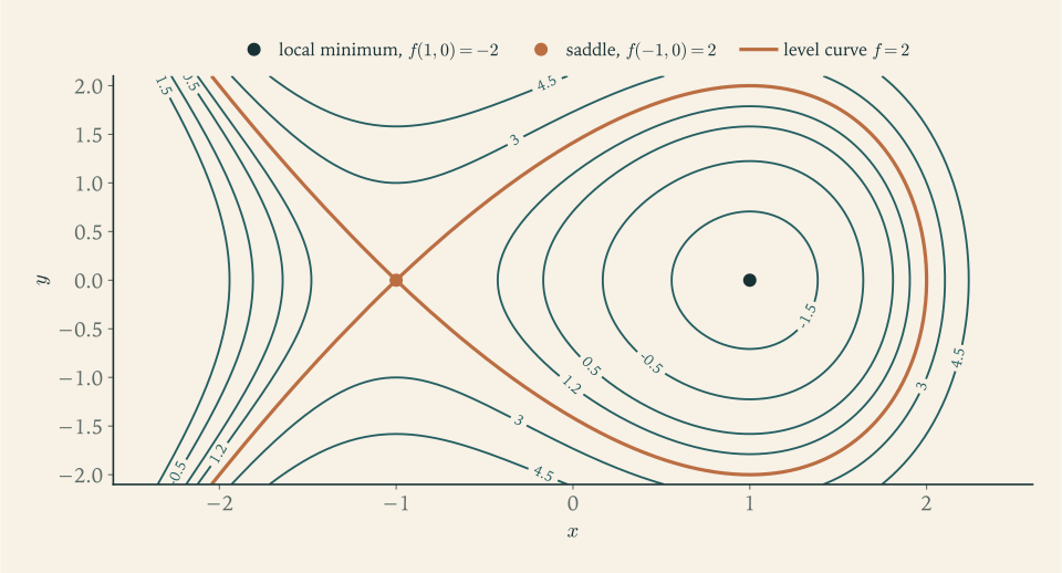
Figure 4.1 shows how the two kinds of critical point look on a contour map. Around the minimum the contours are nested ovals, nearly ellipses whose axes are the eigenvector directions of the Hessian. Through the saddle passes a single self-crossing level curve, \(f=2\) , and the four sectors it cuts out alternate between higher and lower values. One loop of that curve encloses the minimum.
The local minimum is not a global one: \(f(-3,0)=-18\) , far below \(-2\) , and indeed \(f\) is unbounded below as \(x\to-\infty\) . The second derivative test is purely local. It compares \(f(\mathbf a)\) with values at nearby points and knows nothing of what happens far away.
Example 4.3: Local information completed by a global argument
Let \(f(x,y)=x^{4}+y^{4}-4xy\) . The critical point equations \(4x^{3}-4y=0\) and \(4y^{3}-4x=0\) give \(y=x^{3}\) and then \(x=x^{9}\) , so \(x\in\{0,1,-1\}\) , and the critical points are \((0,0)\) , \((1,1)\) , and \((-1,-1)\) . The Hessian is \(\begin{pmatrix}12x^{2}&-4\\ -4&12y^{2}\end{pmatrix}\) . At the origin its determinant is \(-16\) : a saddle. At \((1,1)\) and at \((-1,-1)\) the determinant is \(128\) and \(f_{xx}=12>0\) : two strict local minima, each with value \(f=-2\) .
Are these global minima? The test cannot say, but a separate argument can. Write \(\rho=\lVert(x,y)\rVert\) . Since \(x^{4}+y^{4}\ge\tfrac12(x^{2}+y^{2})^{2}\) and \(4xy\le 2(x^{2}+y^{2})\) , we have \(f\ge\tfrac12\rho^{4}-2\rho^{2}\) , which is nonnegative as soon as \(\rho\ge 2\) . On the closed disc \(\rho\le 2\) the continuous function \(f\) attains a minimum, by the extreme value theorem recalled in Section 4.5. That minimum is at most \(f(1,1)=-2<0\) , so it is not attained on the circle \(\rho=2\) , where \(f\ge 0\) ; it is attained at an interior point, which must be a critical point. Outside the disc \(f\ge 0\) as well. Therefore the global minimum value is \(-2\) , attained at exactly the two points \((1,1)\) and \((-1,-1)\) . The division of labour is typical: an existence argument guarantees that a minimum is somewhere, and the critical point equations say where it can be.
Example 4.4: What a semidefinite Hessian cannot decide
The functions \(x^{4}+y^{4}\) , \(-x^{4}-y^{4}\) , and \(x^{4}-y^{4}\) all have a critical point at the origin with Hessian equal to the zero matrix, which is semidefinite in both senses. The first has a strict minimum there, the second a strict maximum, the third a saddle. So nothing can be concluded from a zero Hessian.
A subtler case is \(f(x,y)=(y-x^{2})(y-3x^{2})\) . Expanding, \(f=y^{2}-4x^{2}y+3x^{4}\) , so the origin is a critical point with \(Hf(0,0)=\begin{pmatrix}0&0\\ 0&2\end{pmatrix}\) , positive semidefinite. Restrict \(f\) to a line \(y=mx\) through the origin:
If \(m\ne 0\) , the last two factors are both close to \(m\) for small \(x\) , so their product is positive and \(f>0\) for all small \(x\ne 0\) . On the line \(y=0\) , \(f=3x^{4}>0\) , and on the line \(x=0\) , \(f=y^{2}>0\) . Along every straight line through the origin, \(f\) has a strict local minimum at the origin.
And yet the origin is not a local minimum of \(f\) . On the parabola \(y=2x^{2}\) , which passes between the two parabolas where the factors vanish, \(f=(x^{2})(-x^{2})\) , which is \(-x^{4}\) , negative at points arbitrarily close to the origin. The region where \(f\) is negative is the thin sliver between \(y=x^{2}\) and \(y=3x^{2}\) ; every line through the origin leaves it immediately, so no line detects it.
Common mistake. Declaring a saddle, or an extremum, when \(D=0\) . The value \(D=0\) means that the quadratic term vanishes in some direction, so that the neglected higher-order terms decide the matter there; it is a statement about the test, not about the function. A related error is to test a critical point only along the coordinate axes or along lines: Example 4.4 shows a function with a minimum along every line and no minimum. When the test is silent, examine the function itself, by factoring, by an inequality, or by finding a curve along which the sign changes.
4.5 Largest and smallest values on a closed bounded set
The second derivative test classifies critical points one at a time. A different and more common question is global: what are the largest and smallest values of \(f\) on a given set \(K\) ? Here the essential fact is an existence theorem from analysis. A subset of \(\mathbb R^n\) is closed if it contains all its boundary points and bounded if it lies in some ball. The fact is the extreme value theorem: a continuous real-valued function on a nonempty closed bounded subset of \(\mathbb R^n\) attains a maximum and a minimum there. Its proof rests on the compactness of closed bounded sets and is given in Real Analysis.
Once existence is known, the extreme points can be hunted down by elimination. An extreme point of \(f\) on \(K\) lies either in the interior of \(K\) or on its boundary. If it is interior and \(f\) is differentiable there, it is a critical point. So the procedure is: find the critical points in the interior; find the extreme values of \(f\) restricted to the boundary, a problem with one variable fewer; then compare the finitely many candidate values. No second derivative test is needed, because we are comparing values, not classifying points.
Example 4.5: Extreme values on a triangle
Find the largest and smallest values of \(f(x,y)=x^{2}+y^{2}-2x-y\) on the closed triangle \(K\) with vertices \((0,0)\) , \((2,0)\) , and \((0,2)\) . The triangle is closed and bounded and \(f\) is continuous, so both extremes are attained.
Interior: \(\nabla f=(2x-2,\ 2y-1)\) vanishes only at \((1,\tfrac12)\) , which lies inside the triangle because \(1+\tfrac12<2\) . There \(f=-\tfrac54\) .
Boundary: there are three edges. On the bottom edge, \(y=0\) and \(f=x^{2}-2x\) for \(0\le x\le 2\) ; its critical point \(x=1\) gives \(-1\) , and the endpoints give \(0\) and \(0\) . On the left edge, \(x=0\) and \(f=y^{2}-y\) for \(0\le y\le 2\) ; its critical point \(y=\tfrac12\) gives \(-\tfrac14\) , and the endpoints give \(0\) and \(2\) . On the slanted edge, put \(x=t\) , \(y=2-t\) with \(0\le t\le 2\) ; then \(f=t^{2}+(2-t)^{2}-2t-(2-t)\) , which simplifies to \(2t^{2}-5t+2\) . Its critical point \(t=\tfrac54\) gives \(-\tfrac98\) , and the endpoints are vertices already counted.
Comparing all candidates, the minimum is \(-\tfrac54\) , at the interior critical point \((1,\tfrac12)\) , and the maximum is \(2\) , at the vertex \((0,2)\) . Since \(f=(x-1)^{2}+(y-\tfrac12)^{2}-\tfrac54\) is the squared distance from \((1,\tfrac12)\) shifted by a constant, the answer has a geometric reading: the minimum is at that point, and the maximum is at the point of the triangle farthest from it.
In the example each edge could be parametrized by a single variable, which reduced the boundary problem to one-variable calculus. For a curved boundary such as a circle or an ellipsoid a parametrization may be awkward or unavailable. The next chapter develops a method that handles a boundary given by an equation without solving the equation. And when the equations \(\nabla f=\mathbf 0\)
cannot be solved by hand at all, one turns to iterative methods that follow the gradient downhill and use the Hessian to choose the step. The first- and second-order optimality conditions for unconstrained problems are taken further in Continuous Optimization (math.continuous-optimization.unconstrained-optimality), where those algorithms are developed.
Exercises
-
State the definition of a critical point, the definition of a positive definite symmetric matrix, and the two-variable form of the second derivative test, including the case in which it gives no conclusion.
-
Compute the Hessian of (a) \(f(x,y)=x^{3}y-xy^{3}\) and (b) \(g(x,y)=\ln(x^{2}+y^{2})\) , verify in each case that the mixed partial derivatives agree, and show that \(g_{xx}+g_{yy}=0\) away from the origin.
Answer
(a) \(f_x=3x^{2}y-y^{3}\) , \(f_y=x^{3}-3xy^{2}\) , and \(Hf=\begin{pmatrix}6xy&3x^{2}-3y^{2}\\ 3x^{2}-3y^{2}&-6xy\end{pmatrix}\) . (b) With \(q=x^{2}+y^{2}\) : \(g_{xx}=2(y^{2}-x^{2})/q^{2}\) , \(g_{yy}=2(x^{2}-y^{2})/q^{2}\) , and \(g_{xy}=g_{yx}=-4xy/q^{2}\) . The two diagonal entries are negatives of each other, so \(g_{xx}+g_{yy}=0\) .
-
Find the second-order Taylor polynomial of \(f(x,y)=\sqrt{1+x+2y}\) at the origin and use it to estimate \(f(0.1,0.05)\) ; compare with the exact value \(\sqrt{1.2}\) .
Answer
With \(w=x+2y\) the polynomial is \(1+\tfrac12w-\tfrac18w^{2}\) , that is, \(1+\tfrac12x+y-\tfrac18(x+2y)^{2}\) . At \((0.1,0.05)\) , \(w=0.2\) and the estimate is \(1+0.1-0.005=1.095\) ; the exact value is \(\sqrt{1.2}\approx 1.09545\) .
-
Classify each symmetric matrix as positive definite, negative definite, indefinite, or semidefinite, using Proposition 4.5: (a) \(\begin{pmatrix}2&1\\ 1&1\end{pmatrix}\) ; (b) \(\begin{pmatrix}1&2\\ 2&1\end{pmatrix}\) ; (c) \(\begin{pmatrix}-3&1\\ 1&-1\end{pmatrix}\) ; (d) \(\begin{pmatrix}1&2\\ 2&4\end{pmatrix}\) .
Answer
(a) \(D=1>0\) and \(a=2>0\) : positive definite. (b) \(D=-3<0\) : indefinite. (c) \(D=2>0\) and \(a=-3<0\) : negative definite. (d) \(D=0\) : positive semidefinite and not definite; the form is \((h+2k)^{2}\) , which vanishes at \((-2,1)\) .
-
Find and classify all critical points of \(f(x,y)=x^{3}+y^{3}-3xy\) , and decide whether \(f\) has a global minimum.
Solution
The gradient is \((3x^{2}-3y,\ 3y^{2}-3x)\) . Setting it to zero gives \(y=x^{2}\) and \(x=y^{2}\) , hence \(x=x^{4}\) , so \(x(x^{3}-1)=0\) and \(x=0\) or \(x=1\) . The critical points are \((0,0)\) and \((1,1)\) .
The Hessian is \(\begin{pmatrix}6x&-3\\ -3&6y\end{pmatrix}\) . At \((0,0)\) its determinant is \(-9\) , which is negative, so the origin is a saddle point. At \((1,1)\) the determinant is \(36-9\) , that is, \(27\) , and \(f_{xx}=6>0\) , so \((1,1)\) is a strict local minimum, with \(f(1,1)=-1\) .
There is no global minimum. Along the negative \(x\) -axis \(f(x,0)=x^{3}\) , which is unbounded below; for instance \(f(-10,0)=-1000\) . So the infimum of \(f\) over the plane is \(-\infty\) and is not attained. Compare Example 4.3, where a growth estimate at infinity turned local minima into global ones; here the cubic terms have no such estimate because they change sign.
-
Find and classify all critical points of \(f(x,y)=xy(1-x-y)\) .
Solution
Expand \(f=xy-x^{2}y-xy^{2}\) . Then \(f_x=y-2xy-y^{2}=y(1-2x-y)\) and \(f_y=x(1-x-2y)\) . From \(f_x=0\) , either \(y=0\) or \(y=1-2x\) . If \(y=0\) , then \(f_y=x(1-x)=0\) gives \((0,0)\) and \((1,0)\) . If \(y=1-2x\) , then \(f_y=x(1-x-2+4x)=x(3x-1)=0\) gives \(x=0\) , \(y=1\) , or \(x=\tfrac13\) , \(y=\tfrac13\) . The four critical points are \((0,0)\) , \((1,0)\) , \((0,1)\) , and \((\tfrac13,\tfrac13)\) .
The Hessian is \(\begin{pmatrix}-2y&1-2x-2y\\ 1-2x-2y&-2x\end{pmatrix}\) . At each of \((0,0)\) , \((1,0)\) , and \((0,1)\) the product of the diagonal entries is zero and the off-diagonal entry is \(\pm1\) , so the determinant is \(-1\) : three saddle points. At \((\tfrac13,\tfrac13)\) the Hessian is \(\begin{pmatrix}-\tfrac23&-\tfrac13\\ -\tfrac13&-\tfrac23\end{pmatrix}\) , with determinant \(\tfrac49-\tfrac19\) , that is, \(\tfrac13\) , and negative upper-left entry: a strict local maximum, with value \(\tfrac13\cdot\tfrac13\cdot\tfrac13\) , that is, \(\tfrac1{27}\) .
The picture explains the count. The function vanishes on the three lines \(x=0\) , \(y=0\) , and \(x+y=1\) , which bound a triangle on which \(f\) is positive. The three saddles are the vertices, where two zero lines cross, and the maximum is inside the triangle.
-
Prove that if \(\begin{pmatrix}a&b\\ b&c\end{pmatrix}\) is positive definite then \(a>0\) and \(c>0\) , and give an example showing that \(a>0\) and \(c>0\) together do not imply positive definiteness.
Hint
Evaluate the quadratic form at \((1,0)\) and at \((0,1)\) . For the counterexample you need \(a>0\) , \(c>0\) , and \(ac-b^{2}<0\) ; part (b) of Exercise 4 is one.
-
Let \(f(x,y)=xy(x^{2}-y^{2})/(x^{2}+y^{2})\) for \((x,y)\ne(0,0)\) and \(f(0,0)=0\) . Compute \(f_x(0,y)\) and \(f_y(x,0)\) , deduce that \(f_{xy}(0,0)=-1\) and \(f_{yx}(0,0)=1\) , and say which hypothesis of Theorem 4.1 must fail.
Solution
Away from the origin \(f\) is a quotient of polynomials with nonvanishing denominator, so all its partial derivatives exist there. On the axes we compute from the definition. For fixed \(y\) and \(h\ne 0\) ,
\[ \frac{f(h,y)-f(0,y)}{h}=\frac{y(h^{2}-y^{2})}{h^{2}+y^{2}}, \]because \(f(0,y)=0\) . As \(h\to 0\) this tends to \(-y\) when \(y\ne 0\) , and it is identically \(0\) when \(y=0\) . So \(f_x(0,y)=-y\) for every \(y\) . In the same way, for fixed \(x\) and \(k\ne 0\) , \((f(x,k)-f(x,0))/k=x(x^{2}-k^{2})/(x^{2}+k^{2})\) , which tends to \(x\) . So \(f_y(x,0)=x\) for every \(x\) .
Now differentiate these one-variable functions at \(0\) . Since \(f_x(0,y)=-y\) , its derivative with respect to \(y\) is \(-1\) , so \(f_{xy}(0,0)=-1\) . Since \(f_y(x,0)=x\) , its derivative with respect to \(x\) is \(1\) , so \(f_{yx}(0,0)=1\) . The mixed partial derivatives at the origin differ.
Theorem 4.1 is not contradicted, so one of its hypotheses fails. The first partial derivatives exist everywhere and the mixed ones exist near the origin, so the failing hypothesis is the continuity of \(f_{xy}\) and \(f_{yx}\) at the origin. Indeed, away from the origin the two mixed derivatives are equal to a common rational function that has no limit at the origin.
-
A student argues: “The function \(f(x,y)=(y-x^{2})(y-3x^{2})\) has a local minimum at the origin along every line through the origin, so it has a local minimum at the origin.” Verify the premise, show that the conclusion is false, and explain what the argument overlooks.
Solution
The premise is true. On the line \(y=mx\) with \(m\ne 0\) , \(f=x^{2}(m-x)(m-3x)\) , and for \(\lvert x\rvert<\lvert m\rvert/3\) both factors \(m-x\) and \(m-3x\) have the sign of \(m\) , so \(f>0\) for small \(x\ne 0\) while \(f=0\) at the origin. On the line \(y=0\) , \(f=3x^{4}\) , and on the line \(x=0\) , \(f=y^{2}\) ; both are positive away from the origin. So the restriction of \(f\) to each line through the origin has a strict local minimum there.
The conclusion is false. On the parabola \(y=2x^{2}\) , \(f=(2x^{2}-x^{2})(2x^{2}-3x^{2})=-x^{4}\) , which is negative for every \(x\ne 0\) . Every ball about the origin contains such points, so \(f(0,0)=0\) is not a local minimum.
What the argument overlooks is that the size of the interval on which each line stays in the region \(f>0\) depends on the line: it is \(\lvert x\rvert<\lvert m\rvert/3\) , which shrinks to nothing as the slope \(m\) tends to \(0\) . A local minimum requires one ball that works for all directions simultaneously. Minimality along every line is a statement about infinitely many one-variable functions, each with its own neighbourhood, and no common neighbourhood need exist. Curved paths can stay inside the thin region between the two parabolas, where \(f<0\) .
-
Find the largest and smallest values of \(f(x,y)=x^{2}-xy+y^{2}-3x\) on the rectangle \(0\le x\le 3\) , \(0\le y\le 2\) .
Solution
The rectangle is closed and bounded and \(f\) is continuous, so both extremes are attained.
Interior: \(f_x=2x-y-3\) and \(f_y=-x+2y\) . Setting both to zero, \(x=2y\) and \(4y-y-3=0\) , so \(y=1\) , \(x=2\) . The point \((2,1)\) is inside the rectangle and \(f(2,1)=4-2+1-6=-3\) .
Edges: on \(y=0\) , \(f=x^{2}-3x\) , with critical value \(-\tfrac94\) at \(x=\tfrac32\) and endpoint values \(0\) and \(0\) . On \(y=2\) , \(f=x^{2}-5x+4\) , with critical value \(-\tfrac94\) at \(x=\tfrac52\) and endpoint values \(4\) at \(x=0\) and \(-2\) at \(x=3\) . On \(x=0\) , \(f=y^{2}\) , increasing from \(0\) to \(4\) . On \(x=3\) , \(f=y^{2}-3y\) , with critical value \(-\tfrac94\) at \(y=\tfrac32\) and endpoint values \(0\) and \(-2\) .
The candidate values are \(-3\) , \(-\tfrac94\) , \(0\) , \(-2\) , and \(4\) . The minimum is \(-3\) at \((2,1)\) , the interior critical point, and the maximum is \(4\) at \((0,2)\) , a corner.
-
Find the line \(y=mx+b\) that minimizes the sum of the squared vertical distances to the points \((0,1)\) , \((1,3)\) , and \((2,4)\) , verify with the Hessian that the critical point is a minimum, and compute the minimal sum of squares.
Solution
The sum of squares is \(S(m,b)=(b-1)^{2}+(m+b-3)^{2}+(2m+b-4)^{2}\) . Its partial derivatives are
\[ S_m=2(m+b-3)+4(2m+b-4)=10m+6b-22,\qquad S_b=2(b-1)+2(m+b-3)+2(2m+b-4)=6m+6b-16 . \]Setting both to zero gives \(5m+3b=11\) and \(3m+3b=8\) . Subtracting, \(2m=3\) , so \(m=\tfrac32\) , and then \(3b=8-\tfrac92\) gives \(b=\tfrac76\) .
The Hessian of \(S\) is the constant matrix \(\begin{pmatrix}10&6\\ 6&6\end{pmatrix}\) , with determinant \(24>0\) and positive upper-left entry, so it is positive definite and the critical point is a strict local minimum. Because \(S\) is a quadratic polynomial, the first formula of Theorem 4.3 holds exactly with this constant Hessian, so \(S(m,b)\) exceeds its value at the critical point by a positive definite quadratic form in the displacement: the minimum is global.
The residuals at the three points are \(b-1=\tfrac16\) , \(m+b-3=-\tfrac13\) , and \(2m+b-4=\tfrac16\) , so the minimal sum of squares is \(\tfrac1{36}+\tfrac4{36}+\tfrac1{36}\) , that is, \(\tfrac16\) . The best line is \(y=\tfrac32x+\tfrac76\) .
-
Let \(f\) be of class \(C^2\) and suppose \(f\) has a local minimum at an interior point \(\mathbf a\) . Prove that \(Hf(\mathbf a)\) is positive semidefinite.
Solution
Since \(\mathbf a\) is an interior local minimum of a differentiable function, \(\nabla f(\mathbf a)=\mathbf 0\) . Suppose, for contradiction, that \(H=Hf(\mathbf a)\) is not positive semidefinite. Then there is a vector \(\mathbf v\) with \(\mathbf v^{\top}H\mathbf v<0\) . By Theorem 4.3, for small \(t\ne 0\) ,
\[ f(\mathbf a+t\mathbf v)-f(\mathbf a)=t^{2}\Bigl(\tfrac12\mathbf v^{\top}H\mathbf v+\frac{R(t\mathbf v)}{t^{2}}\Bigr), \]and \(R(t\mathbf v)/t^{2}\to 0\) as \(t\to 0\) . The bracket therefore tends to the negative number \(\tfrac12\mathbf v^{\top}H\mathbf v\) , so it is negative for all sufficiently small \(t\ne 0\) . For those \(t\) we get \(f(\mathbf a+t\mathbf v)<f(\mathbf a)\) , at points as close to \(\mathbf a\) as we please. That contradicts the assumption of a local minimum. Hence \(\mathbf v^{\top}H\mathbf v\ge 0\) for every \(\mathbf v\) .
The result is a necessary condition and cannot be strengthened to positive definiteness: \(x^{4}+y^{4}\) has a minimum at the origin with zero Hessian. Nor is it sufficient: Example 4.4 has a positive semidefinite Hessian at a point that is not a minimum.
-
For which values of the constant \(k\) does \(f(x,y)=x^{2}+kxy+y^{2}\) have a strict local minimum at the origin, for which a saddle, and what happens in the remaining cases?
Hint
The Hessian is \(\begin{pmatrix}2&k\\ k&2\end{pmatrix}\) with \(D=4-k^{2}\) . Apply Proposition 4.5 for \(\lvert k\rvert<2\) and \(\lvert k\rvert>2\) . For \(k=\pm 2\) the test is silent, but the function is a perfect square, \((x\pm y)^{2}\) : decide directly whether the origin is a minimum and whether it is strict.
-
Show that the origin is the only critical point of \(f(x,y,z)=x^{2}+y^{2}+z^{2}+xy+yz\) , write down the Hessian, and classify the critical point using the eigenvalue criterion of Section 4.3.
Hint
The gradient is \((2x+y,\ x+2y+z,\ y+2z)\) , a linear system with matrix \(H=\begin{pmatrix}2&1&0\\ 1&2&1\\ 0&1&2\end{pmatrix}\) , which is also the Hessian. Its determinant is \(4\) , so the only solution is the origin. The eigenvalues are \(2\) and \(2\pm\sqrt2\) , all positive.
-
A contour map of a \(C^2\) function shows nested closed level curves around a point \(P\) with values decreasing toward \(P\) , and a level curve that crosses itself at a point \(Q\) . Say what the picture establishes about \(P\) and about \(Q\) , what further information about the values near \(Q\) would settle its type, and what can and cannot be concluded about the eigenvalues of the Hessian at each.
Solution
\(P\) is a local minimum: values decrease toward it from every side. The Hessian there is positive semidefinite by Exercise 12, but the picture cannot show that it is positive definite; \(x^{4}+y^{4}\) has the same kind of contour map with a zero Hessian.
\(Q\) is a critical point. If the gradient at \(Q\) were not zero, the implicit function theorem, Theorem 3.6, would make the level set near \(Q\) the graph of a single \(C^1\) function of one of the variables, and a graph cannot cross itself. That is all the crossing establishes. It does not make \(Q\) a saddle: for \(x^{2}y^{2}\) the level set through the origin is the pair of coordinate axes, which cross there, and the origin is a minimum.
What settles the type is the values of the function in the sectors that the crossing curve cuts out near \(Q\) . If they are higher than \(f(Q)\) in some sectors and lower in others, as at \((-1,0)\) in Figure 4.1 where the four sectors alternate, then \(Q\) is a saddle. If they are all higher, or all lower, \(Q\) is a local extremum.
About the Hessian at \(Q\) the picture says little. If \(Q\) is a saddle and the Hessian is invertible, its eigenvalues have opposite signs; but a saddle can also have a degenerate Hessian, and in the example \(x^{2}y^{2}\) the Hessian at the crossing point is zero.
-
The lines \(\mathbf p(s)=(s,0,0)\) and \(\mathbf q(t)=(1,t,t+1)\) do not meet. Find the distance between them by minimizing the squared distance between \(\mathbf p(s)\) and \(\mathbf q(t)\) over \((s,t)\) , and check the answer using the cross product of the two direction vectors from Chapter 1.
Solution
The squared distance between \(\mathbf p(s)\) and \(\mathbf q(t)\) is
\[ d^{2}(s,t)=(s-1)^{2}+(0-t)^{2}+(0-t-1)^{2}=(s-1)^{2}+t^{2}+(t+1)^{2}. \]Its partial derivatives are \(2(s-1)\) and \(2t+2(t+1)=4t+2\) , which vanish at \(s=1\) , \(t=-\tfrac12\) . The Hessian is the diagonal matrix with entries \(2\) and \(4\) , positive definite, and \(d^{2}\) is a quadratic polynomial, so this critical point is the global minimum. The minimal value is \(0+\tfrac14+\tfrac14=\tfrac12\) , and the distance between the lines is \(1/\sqrt2\) . The closest points are \((1,0,0)\) and \((1,-\tfrac12,\tfrac12)\) .
For the check, the shortest segment between two lines is perpendicular to both, so it is parallel to the cross product of the directions: \((1,0,0)\times(0,1,1)=(0,-1,1)\) . The distance is the absolute value of the component along this vector of any vector joining the lines, say \(\mathbf q(0)-\mathbf p(0)=(1,0,1)\) : it is \(\lvert(1,0,1)\cdot(0,-1,1)\rvert/\sqrt2=1/\sqrt2\) . Indeed the segment joining the closest points, \((0,-\tfrac12,\tfrac12)\) , is a multiple of \((0,-1,1)\) .
-
Show that \(f(x,y)=x^{2}+y^{2}(1-x)^{3}\) has exactly one critical point, that it is a strict local minimum, and that \(f\) nevertheless has no global minimum. Why is this impossible for a differentiable function of one variable?
Solution
The partial derivatives are \(f_x=2x-3y^{2}(1-x)^{2}\) and \(f_y=2y(1-x)^{3}\) . From \(f_y=0\) , either \(y=0\) or \(x=1\) . If \(x=1\) then \(f_x=2\ne 0\) , so there is no critical point on that line. If \(y=0\) then \(f_x=2x=0\) gives \(x=0\) . The only critical point is the origin.
At the origin \(f_{xx}=2\) , \(f_{xy}=-6y(1-x)^{2}=0\) , and \(f_{yy}=2(1-x)^{3}=2\) , so the Hessian is twice the identity matrix, positive definite. The origin is a strict local minimum, with \(f=0\) .
But on the vertical line \(x=4\) the function is \(16-27y^{2}\) , which tends to \(-\infty\) as \(y\to\pm\infty\) . So \(f\) takes values below \(0\) and is unbounded below: no global minimum exists.
In one variable this cannot happen. If a differentiable function on the line has a strict local minimum at \(a\) and takes a smaller value at some point \(b\) , then on the closed interval between \(a\) and \(b\) it attains a maximum, and that maximum is at an interior point because the function rises on leaving \(a\) and is below \(f(a)\) at \(b\) ; there the derivative vanishes, giving a second critical point. In two variables one can walk around a hill instead of over it, and no second critical point is forced.
-
For \(f(x,y)=x^{2}y\) , \(\mathbf a=(1,1)\) , and \(\mathbf v=(1,2)\) , let \(g(t)=f(\mathbf a+t\mathbf v)\) . Compute \(g''(0)\) from the formula \(\mathbf v^{\top}Hf(\mathbf a)\mathbf v\) in the proof of Theorem 4.3, and check by expanding \(g\) as a polynomial in \(t\) .
Answer
\(Hf=\begin{pmatrix}2y&2x\\ 2x&0\end{pmatrix}\) , which at \((1,1)\) is \(\begin{pmatrix}2&2\\ 2&0\end{pmatrix}\) , and \(\mathbf v^{\top}Hf(\mathbf a)\mathbf v=2+4+4+0=10\) . Directly, \(g(t)=(1+t)^{2}(1+2t)=1+4t+5t^{2}+2t^{3}\) , so \(g''(0)=10\) .