Among all points \((x,y)\) on the ellipse \(x^{2}+4y^{2}=8\) , which make the product \(xy\) largest? The gradient of \(xy\) is \((y,x)\) , which vanishes only at the origin, and the origin is not on the ellipse. So the method of Chapter 4 finds nothing: there are no critical points to examine. And yet the ellipse is closed and bounded and \(xy\) is continuous, so a largest value certainly exists.

The difficulty is that the candidates of Chapter 4 are the points where \(f\) cannot be increased by moving in any direction. On the ellipse we are not allowed to move in any direction, only along the curve. A maximum on the curve is a point where \(f\) cannot be increased by an allowed move, which is a weaker requirement and needs its own condition. One could parametrize the ellipse and reduce to one variable, as in Example 4.5. The method of this chapter avoids parametrizing altogether. It works directly with the equation of the constraint, in any number of variables, and it attaches to each solution a number, the multiplier, that turns out to have a meaning of its own.

5.1 Why the gradients must line up

Write the constraint as \(g(x,y)=c\) with \(g=x^{2}+4y^{2}\) , and picture the level curves of \(f=xy\) drawn over the ellipse. Where a level curve \(f=k\) crosses the ellipse transversally, walking along the ellipse carries us from the side where \(f<k\) to the side where \(f>k\) . So \(f\) is still increasing along the ellipse at such a point, and the point is not a maximum. At a maximum the level curve of \(f\) through the point cannot cross the ellipse; the two curves must touch.

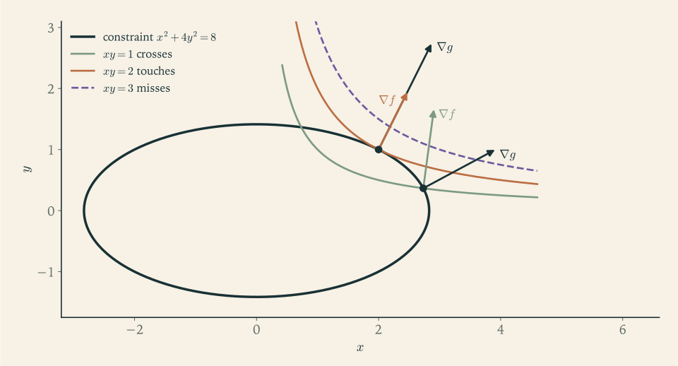
Figure 5.1 shows the three possibilities. The curve \(xy=1\) crosses the ellipse, so the value \(1\) can be improved. The curve \(xy=3\) does not meet the ellipse, so the value \(3\) is not available. The curve \(xy=2\) touches the ellipse at \((2,1)\) , and \(2\) is the maximum. Now recall Corollary 2.11: the gradient of a function is perpendicular to its level curves. Two curves that are tangent at a point have the same tangent line there, hence the same normal line, so \(\nabla f\) and \(\nabla g\) are parallel at the point of tangency. In the figure the two arrows at \((2,1)\) lie along one line, while at the crossing point they do not.

The same conclusion can be reached without a picture, in a form that generalizes. Let \(\mathbf r(t)\) be any differentiable curve that stays in the constraint set and passes through a constrained maximum \(\mathbf a\) at \(t=0\) . Then \(t\mapsto f(\mathbf r(t))\) has a maximum at \(t=0\) , so its derivative there is zero, and by Theorem 2.10 that derivative is \(\nabla f(\mathbf a)\cdot\mathbf r'(0)\) . So \(\nabla f(\mathbf a)\) is orthogonal to the velocity of every curve in the constraint set through \(\mathbf a\) . By Corollary 2.11 so is \(\nabla g(\mathbf a)\) . If the velocities of such curves fill out everything orthogonal to \(\nabla g(\mathbf a)\) , a vector orthogonal to all of them must be a multiple of \(\nabla g(\mathbf a)\) . That “if” is where the implicit function theorem enters, and it is why the theorem below has a hypothesis on \(\nabla g\) .

5.2 The multiplier rule

The proof makes the role of each hypothesis visible. Regularity of the point is what allows the constraint to be solved locally for one variable. The constrained problem then becomes an unconstrained one in the remaining variables, to which the result of Chapter 2 applies, and the multiplier appears as the ratio that makes the bookkeeping symmetric in all the variables. The point of the theorem is that we never have to find \(\varphi\) .

The theorem gives a necessary condition. It does not say that a constrained extremum exists, and it does not say that a point satisfying the condition is one. In use, it is a way of producing a short list of candidates:

To find the extreme values of \(f\) on \(S=\{g=c\}\) , first decide whether they exist, usually by observing that \(S\) is closed and bounded and invoking the extreme value theorem. Then solve the \(n+1\) equations \(\nabla f=\lambda\nabla g\) , \(g=c\) for the \(n+1\) unknowns \(x_1,\dots,x_n,\lambda\) . Add to the list any points of \(S\) where \(\nabla g=\mathbf 0\) , since the theorem says nothing about them. Finally evaluate \(f\) at every point on the list and compare.

5.3 The method at work

5.4 When the rule misses the answer

Theorem 5.2 has three hypotheses: smoothness, the existence of an extremum, and regularity of the point. Each can fail, and when one does, the list of solutions of the multiplier equations can be incomplete or misleading.

5.5 What the multiplier measures

The multiplier is usually eliminated on the way to the solution and then forgotten. It deserves better. Suppose the constraint level \(c\) is a resource, a budget or a length of fence, and ask how the optimal value changes when the resource changes.

So \(\lambda\) is the marginal value of the constraint: the amount by which the optimum improves per unit relaxation of the constraint level. In economics it is called a shadow price.

5.6 Quadratic forms on the unit sphere

The multiplier rule gives a short proof of a fact used in Section 4.3, and explains why eigenvalues were the right tool there.

The multiplier here is the eigenvalue, and by Theorem 5.3 with \(c=\lVert\mathbf x\rVert^{2}\) it is the rate at which the extreme value of the form grows with the squared radius of the sphere.

5.7 Several constraints, and regions with boundary

A curve in space is typically the intersection of two surfaces, and optimizing along it means imposing two constraints at once.

The proof follows the pattern of Theorem 5.2, with the implicit function theorem for a pair of equations solving for two of the variables; that version of the theorem is proved in analysis courses, and we use the result without reproducing the argument. The geometric content is the same as before. The gradient of \(f\) must be orthogonal to the constraint curve, and the vectors orthogonal to the curve are the combinations of the two normals \(\nabla g\) and \(\nabla h\) . Linear independence of the two normals is the regularity condition: it says the two surfaces cross transversally and do not merely touch.

Exercises

1. State the Lagrange multiplier rule with all of its hypotheses, and for each hypothesis name an example from this chapter in which the conclusion or its usefulness fails when the hypothesis is dropped.

2. Find the largest and smallest values of \(f(x,y)=3x+4y\) on the circle \(x^{2}+y^{2}=25\) , the points where they occur, and the value of the multiplier at each.

   Answer

   The equations \(3=2\lambda x\) , \(4=2\lambda y\) give \((x,y)\) proportional to \((3,4)\) . The maximum is \(25\) at \((3,4)\) with \(\lambda=\tfrac12\) ; the minimum is \(-25\) at \((-3,-4)\) with \(\lambda=-\tfrac12\) .

3. Find the largest and smallest values of \(f(x,y)=x^{2}y\) on the ellipse \(x^{2}+2y^{2}=6\) , treating separately any case in which you would otherwise divide by zero.

   Solution

   The ellipse is closed and bounded, so both extremes exist, and \(\nabla g=(2x,4y)\) with \(g=x^{2}+2y^{2}\) vanishes only at the origin, which is not on the ellipse. The multiplier equations are

   \[ 2xy=2\lambda x,\qquad x^{2}=4\lambda y,\qquad x^{2}+2y^{2}=6 . \]

   The first equation is \(2x(y-\lambda)=0\) , so either \(x=0\) or \(y=\lambda\) . These two cases must be kept apart; dividing by \(x\) would lose the first.

   Case \(x=0\) : the constraint gives \(y=\pm\sqrt3\) , and the second equation is satisfied with \(\lambda=0\) . At these points \(f=0\) .

   Case \(y=\lambda\) : the second equation becomes \(x^{2}=4y^{2}\) , and the constraint gives \(4y^{2}+2y^{2}=6\) , so \(y=\pm 1\) and \(x=\pm 2\) . At \((\pm 2,1)\) , \(f=4\) ; at \((\pm 2,-1)\) , \(f=-4\) .

   Comparing the candidate values \(0\) , \(4\) , and \(-4\) : the maximum is \(4\) , attained at \((2,1)\) and \((-2,1)\) , and the minimum is \(-4\) , attained at \((2,-1)\) and \((-2,-1)\) . The points with \(x=0\) are neither; they are the places where \(f\) , which has the sign of \(y\) , passes through a local extreme value of \(0\) along the top and bottom of the ellipse.

4. A rectangular box with faces parallel to the coordinate planes is inscribed in the ellipsoid \(x^{2}/a^{2}+y^{2}/b^{2}+z^{2}/c^{2}=1\) . Use a multiplier to find the largest possible volume.

   Hint

   Let \((x,y,z)\) be the corner in the first octant, so the volume is \(8xyz\) . Write the three multiplier equations, multiply the first by \(x\) , the second by \(y\) , the third by \(z\) , and compare: you should find \(x^{2}/a^{2}=y^{2}/b^{2}=z^{2}/c^{2}\) , each equal to \(\tfrac13\) by the constraint. The largest volume is \(8abc/(3\sqrt3)\) .

5. Use the multiplier rule to find the point of the plane \(2x-y+2z=9\) closest to the origin, justifying the existence of a closest point, and check the distance against the point-to-plane formula of Chapter 1.

   Solution

   Minimize \(f=x^{2}+y^{2}+z^{2}\) , the squared distance to the origin, subject to \(g=2x-y+2z=9\) . For existence: the plane is closed, and on it \(f\) exceeds any given bound outside a large enough ball, so the minimum over the plane equals the minimum over the part of the plane inside that ball, a closed bounded set, where it is attained.

   \(\nabla g=(2,-1,2)\) is never zero. The multiplier equations \(2x=2\lambda\) , \(2y=-\lambda\) , \(2z=2\lambda\) give \((x,y,z)=\tfrac\lambda2(2,-1,2)\) . Substituting into the constraint, \(\tfrac\lambda2(4+1+4)=9\) , so \(\lambda=2\) and the point is \((2,-1,2)\) . It is the only candidate, so it is the closest point, and its distance from the origin is \(\sqrt{4+1+4}\) : the distance is \(3\) .

   The formula of Chapter 1 gives the distance from the origin to the plane \(\mathbf n\cdot\mathbf x=9\) with \(\mathbf n=(2,-1,2)\) as \(\lvert 0-9\rvert/\lVert\mathbf n\rVert=9/3=3\) , in agreement. The multiplier solution also shows that the closest point is a multiple of the normal, as geometry demands.

6. Let \(s>0\) . Prove that the maximum of \(xyz\) over \(x,y,z\ge 0\) with \(x+y+z=s\) is \((s/3)^{3}\) , and deduce the inequality \(\sqrt[3]{xyz}\le(x+y+z)/3\) for nonnegative numbers.

   Solution

   Let \(K\) be the set of points with \(x,y,z\ge 0\) and \(x+y+z=s\) . It is closed and bounded, and \(xyz\) is continuous, so a maximum exists. On the part of \(K\) where some coordinate is zero the product is \(0\) , while \(K\) contains points with all coordinates positive, where the product is positive. So the maximum is attained at a point \(\mathbf a\) with \(x,y,z>0\) .

   Near such a point the conditions \(x,y,z\ge 0\) are not binding, so \(\mathbf a\) is a local maximum of \(f=xyz\) on the plane \(g=x+y+z=s\) , and \(\nabla g=(1,1,1)\ne\mathbf 0\) . Theorem 5.2 gives

   \[ yz=\lambda,\qquad xz=\lambda,\qquad xy=\lambda . \]

   From the first two, \(yz=xz\) , and since \(z>0\) , \(x=y\) . From the last two, \(y=z\) . So \(x=y=z=s/3\) , and this is the only candidate with positive coordinates. Hence the maximum is \((s/3)^{3}\) .

   Now let \(x,y,z\) be any nonnegative numbers and put \(s=x+y+z\) . If \(s=0\) all three vanish and the inequality is trivial. Otherwise \((x,y,z)\in K\) , so \(xyz\le(s/3)^{3}\) , and taking cube roots gives \(\sqrt[3]{xyz}\le(x+y+z)/3\) . Equality holds only at the maximizer, that is, when the three numbers are equal.

7. Find the point of the curve \((x-1)^{3}=y^{2}\) closest to the origin. Show that the multiplier equations have no solution, and explain why this does not contradict Theorem 5.2.

   Solution

   Minimize \(f=x^{2}+y^{2}\) subject to \(g=(x-1)^{3}-y^{2}=0\) . On the curve \((x-1)^{3}=y^{2}\ge 0\) , so \(x\ge 1\) and therefore \(f\ge 1\) , with equality exactly at \((1,0)\) , which is on the curve. The closest point is \((1,0)\) and the minimum value is \(1\) .

   The multiplier equations are \(2x=3\lambda(x-1)^{2}\) and \(2y=-2\lambda y\) together with the constraint. The second equation gives \(y=0\) or \(\lambda=-1\) . If \(y=0\) the constraint forces \(x=1\) , and the first equation becomes \(2=0\) , which is false. If \(\lambda=-1\) the first equation is \(2x=-3(x-1)^{2}\) , that is, \(3x^{2}-4x+3=0\) , whose discriminant \(16-36\) is negative. So the system has no real solution.

   There is no contradiction with Theorem 5.2, because the theorem applies only at regular points. Here \(\nabla g=(3(x-1)^{2},-2y)\) vanishes at \((1,0)\) , the very point where the minimum occurs. The curve has a cusp there. The correct procedure adds the singular points of the constraint to the candidate list, and then the list consists of the single point \((1,0)\) .

8. A student maximizing and minimizing \(f(x,y)=x+y\) on the hyperbola \(xy=1\) finds the multiplier solutions \((1,1)\) and \((-1,-1)\) and reports “maximum \(2\) , minimum \(-2\) ”. Explain every error in this report and describe the true behaviour of \(f\) on the hyperbola.

   Solution

   There are two errors. First, the report assumes that a maximum and a minimum exist. The hyperbola is closed but not bounded, so the extreme value theorem does not apply, and in fact neither exists: taking \(x=t\) , \(y=1/t\) with \(t\to+\infty\) makes \(f=t+1/t\) arbitrarily large, and taking \(t\to-\infty\) makes it arbitrarily negative.

   Second, even as a description of local behaviour the report has the roles reversed. On the branch \(x>0\) we have \(f=x+1/x\) , whose derivative \(1-1/x^{2}\) is negative for \(x<1\) and positive for \(x>1\) ; so \((1,1)\) is a local minimum of \(f\) on the hyperbola, with value \(2\) , and it is the smallest value on that branch. On the branch \(x<0\) the same computation shows that \((-1,-1)\) is a local maximum, with value \(-2\) , the largest value on that branch.

   So the true picture is: \(f\) takes every value in \([2,\infty)\) on one branch and every value in \((-\infty,-2]\) on the other; it has a local minimum equal to \(2\) , a local maximum equal to \(-2\) , and no global extremes. The multiplier rule found exactly the points it is entitled to find, the constrained local extrema. The mistake lay in comparing their values as though one list of candidates on a bounded set were being ranked.

9. Find the largest and smallest values of \(f(x,y,z)=x+y+z\) on the curve in which the cylinder \(x^{2}+y^{2}=2\) meets the plane \(x+z=1\) , using two multipliers and checking the linear-independence hypothesis.

   Solution

   Let \(g=x^{2}+y^{2}\) and \(h=x+z\) , so \(\nabla g=(2x,2y,0)\) and \(\nabla h=(1,0,1)\) . These are linearly dependent only if \((2x,2y,0)\) is a multiple of \((1,0,1)\) , which forces \(x=y=0\) ; no such point is on the cylinder. So Theorem 5.5 applies at every point of the curve, and the curve is closed and bounded, so both extremes exist.

   With \(\nabla f=(1,1,1)\) the condition \(\nabla f=\lambda\nabla g+\mu\nabla h\) reads

   \[ 1=2\lambda x+\mu,\qquad 1=2\lambda y,\qquad 1=\mu . \]

   So \(\mu=1\) , and the first equation becomes \(2\lambda x=0\) . The second shows \(\lambda\ne 0\) , hence \(x=0\) . The cylinder gives \(y=\pm\sqrt2\) and the plane gives \(z=1\) . The candidates are \((0,\sqrt2,1)\) , where \(f=1+\sqrt2\) , and \((0,-\sqrt2,1)\) , where \(f=1-\sqrt2\) . These are the maximum and the minimum.

   As a check, on the curve \(z=1-x\) , so \(f=x+y+1-x=1+y\) , and \(y\) ranges over \([-\sqrt2,\sqrt2]\) on the cylinder.

10. Find the largest and smallest values of \(f(x,y)=2x^{2}+3y^{2}-4x-5\) on the disc \(x^{2}+y^{2}\le 16\) .

    Solution

    The disc is closed and bounded, so the extremes exist.

    Interior: \(\nabla f=(4x-4,\ 6y)\) vanishes only at \((1,0)\) , which is inside the disc; \(f(1,0)=2-4-5=-7\) .

    Boundary: with \(g=x^{2}+y^{2}=16\) the multiplier equations are \(4x-4=2\lambda x\) and \(6y=2\lambda y\) . The second gives \(y=0\) or \(\lambda=3\) . If \(y=0\) , then \(x=\pm 4\) : \(f(4,0)=32-16-5=11\) and \(f(-4,0)=32+16-5=43\) . If \(\lambda=3\) , the first gives \(4x-4=6x\) , so \(x=-2\) and \(y^{2}=12\) ; then \(f=8+36+8-5=47\) .

    Comparing \(-7\) , \(11\) , \(43\) , and \(47\) : the maximum is \(47\) , at \((-2,\pm2\sqrt3)\) , and the minimum is \(-7\) , at the interior critical point \((1,0)\) . Note that the largest boundary value is not at the point \((-4,0)\) farthest from the interior minimum; the coefficient \(3\) of \(y^{2}\) makes it worthwhile to trade some \(x\) for \(y\) .

11. For the problem of Exercise 2 with the radius allowed to vary, let \(M(c)\) be the maximum of \(3x+4y\) on \(x^{2}+y^{2}=c\) . Find \(M(c)\) , verify that \(M'(25)\) equals the multiplier found in Exercise 2, and use the multiplier to estimate \(M(26)\) .

    Answer

    \(M(c)=5\sqrt c\) , so \(M'(c)=5/(2\sqrt c)\) and \(M'(25)=\tfrac12\) , the multiplier of Exercise 2. The estimate is \(M(26)\approx 25+\tfrac12=25.5\) ; the exact value is \(5\sqrt{26}\approx 25.495\) .

12. A consumer’s satisfaction from quantities \(x\) and \(y\) of two goods is \(U(x,y)=x^{1/3}y^{2/3}\) . The first good costs \(2\) units of money each, the second costs \(1\) , and the budget is \(12\) . Formulate the problem of maximizing \(U\) with the whole budget spent, solve it with a multiplier, and interpret the multiplier.

    Answer

    Maximize \(U=x^{1/3}y^{2/3}\) subject to \(2x+y=12\) . The equations \(U_x=2\lambda\) , \(U_y=\lambda\) give \(U_x=2U_y\) , that is, \(y=4x\) ; with the budget, \(x=2\) and \(y=8\) , and \(U=2^{1/3}\cdot 4\approx 5.04\) . The multiplier is \(\lambda=U_y(2,8)=\tfrac23(2/8)^{1/3}\approx 0.42\) : one more unit of budget raises the attainable satisfaction by about \(0.42\) .

13. Find the largest and smallest values of \(q(x,y)=x^{2}+4xy+y^{2}\) on the unit circle by identifying them as eigenvalues of a matrix, and state where they are attained.

    Answer

    \(q=\mathbf x^{\top}A\mathbf x\) with \(A=\begin{pmatrix}1&2\\ 2&1\end{pmatrix}\) , whose eigenvalues are \(3\) and \(-1\) . The maximum is \(3\) , at \(\pm(1,1)/\sqrt2\) ; the minimum is \(-1\) , at \(\pm(1,-1)/\sqrt2\) .

14. Let \(S=\{g=c\}\) where \(g\) is \(C^1\) , let \(\mathbf p\) be a point not on \(S\) , and suppose \(\mathbf q\) is a point of \(S\) closest to \(\mathbf p\) with \(\nabla g(\mathbf q)\ne\mathbf 0\) . Prove that \(\mathbf p-\mathbf q\) is parallel to \(\nabla g(\mathbf q)\) .

    Solution

    Consider \(f(\mathbf x)=\lVert\mathbf x-\mathbf p\rVert^{2}=(\mathbf x-\mathbf p)\cdot(\mathbf x-\mathbf p)\) , a polynomial in the coordinates and therefore of class \(C^1\) , with gradient \(\nabla f(\mathbf x)=2(\mathbf x-\mathbf p)\) . Since \(\mathbf q\) is a point of \(S\) closest to \(\mathbf p\) , it minimizes the distance and hence the squared distance over \(S\) ; in particular \(f\) has a local minimum on \(S\) at \(\mathbf q\) . By hypothesis \(g\) is \(C^1\) and \(\nabla g(\mathbf q)\ne\mathbf 0\) , so \(\mathbf q\) is a regular point and Theorem 5.2 applies: there is a number \(\lambda\) with

    \[ 2(\mathbf q-\mathbf p)=\lambda\,\nabla g(\mathbf q). \]

    Thus \(\mathbf p-\mathbf q=-\tfrac\lambda2\nabla g(\mathbf q)\) is a multiple of \(\nabla g(\mathbf q)\) . Because \(\mathbf p\) is not on \(S\) , \(\mathbf p\ne\mathbf q\) , so the multiple is nonzero and the two vectors are genuinely parallel. In words: the shortest segment from a point to a smooth surface meets the surface at a right angle, since \(\nabla g(\mathbf q)\) is normal to \(S\) by Corollary 2.11. Examples 5.2 and Exercise 5 are special cases.

15. A closed cylindrical can is to hold a fixed volume \(V\) . Use a multiplier to show that the surface area is smallest when the height equals the diameter.

    Hint

    Minimize \(A=2\pi r^{2}+2\pi rh\) subject to \(\pi r^{2}h=V\) . The equation from \(\partial/\partial h\) gives \(\lambda=2/r\) ; substitute into the equation from \(\partial/\partial r\) to get \(h=2r\) . For existence, note that \(A\to\infty\) both as \(r\to 0\) and as \(r\to\infty\) along the constraint.

16. To find the extremes of \(f(x,y)=y^{2}-x^{2}\) on the unit circle, a student writes \(-2x=2\lambda x\) , divides by \(x\) to get \(\lambda=-1\) , deduces \(y=0\) from \(2y=2\lambda y\) , and concludes that the only candidates are \((\pm1,0)\) , where \(f=-1\) , so that \(f\) is constant on the circle. Find the error and give the correct maximum and minimum.

    Solution

    The error is the division by \(x\) in the equation \(-2x=2\lambda x\) . That equation is \(2x(\lambda+1)=0\) , which has two kinds of solution: \(\lambda=-1\) , or \(x=0\) . Dividing by \(x\) silently assumes \(x\ne 0\) and discards the second kind.

    Treat both cases. If \(\lambda=-1\) , the other equation \(2y=2\lambda y\) becomes \(4y=0\) , so \(y=0\) and \(x=\pm 1\) , where \(f=-1\) . If \(x=0\) , the constraint gives \(y=\pm 1\) , and the equation \(2y=2\lambda y\) holds with \(\lambda=1\) ; at \((0,\pm1)\) , \(f=1\) .

    The circle is closed and bounded, so the extremes exist and are among the four candidates: the maximum is \(1\) , at \((0,\pm 1)\) , and the minimum is \(-1\) , at \((\pm 1,0)\) . The student’s conclusion that \(f\) is constant on the circle should itself have raised suspicion, since \(f(0,1)=1\) can be computed directly. On the circle \(f=1-2x^{2}\) , which confirms the answer.

17. Find the largest and smallest values of \(f(x,y)=x^{2}+xy+y^{2}\) on the disc \(x^{2}+y^{2}\le 8\) , using the second derivative test of Chapter 4 for the interior and Proposition 5.4 for the boundary.

    Hint

    In the interior the only critical point is the origin, where the Hessian \(\begin{pmatrix}2&1\\ 1&2\end{pmatrix}\) is positive definite and \(f=0\) . On the boundary write \(f=\mathbf x^{\top}A\mathbf x\) with \(A=\begin{pmatrix}1&\tfrac12\\ \tfrac12&1\end{pmatrix}\) , whose eigenvalues are \(\tfrac32\) and \(\tfrac12\) ; on a circle of squared radius \(8\) the form ranges between \(4\) and \(12\) . The maximum is \(12\) , at \(\pm(2,2)\) , and the minimum is \(0\) , at the origin.

18. Let \(\mathbf a\in\mathbb R^n\) be a nonzero vector. Use the multiplier rule to find the maximum of \(\mathbf a\cdot\mathbf x\) over the unit sphere \(\lVert\mathbf x\rVert=1\) , show that the result recovers the Cauchy–Schwarz inequality of Chapter 1, and say whether this counts as an independent proof of that inequality.

    Solution

    The unit sphere is closed and bounded and \(f(\mathbf x)=\mathbf a\cdot\mathbf x\) is continuous, so a maximum exists. With \(g(\mathbf x)=\mathbf x\cdot\mathbf x\) we have \(\nabla f=\mathbf a\) and \(\nabla g=2\mathbf x\) , nonzero on the sphere. The multiplier rule gives \(\mathbf a=2\lambda\mathbf x\) . Since \(\mathbf a\ne\mathbf 0\) , \(\lambda\ne 0\) and \(\mathbf x=\mathbf a/(2\lambda)\) ; the constraint \(\lVert\mathbf x\rVert=1\) forces \(2\lambda=\pm\lVert\mathbf a\rVert\) . The two candidates are \(\mathbf x=\pm\mathbf a/\lVert\mathbf a\rVert\) , with values \(\pm\lVert\mathbf a\rVert\) . So the maximum of \(\mathbf a\cdot\mathbf x\) on the unit sphere is \(\lVert\mathbf a\rVert\) and the minimum is \(-\lVert\mathbf a\rVert\) .

    Now let \(\mathbf b\) be any nonzero vector. The unit vector \(\mathbf b/\lVert\mathbf b\rVert\) lies on the sphere, so \(-\lVert\mathbf a\rVert\le\mathbf a\cdot\mathbf b/\lVert\mathbf b\rVert\le\lVert\mathbf a\rVert\) , that is, \(\lvert\mathbf a\cdot\mathbf b\rvert\le\lVert\mathbf a\rVert\lVert\mathbf b\rVert\) , with equality only when \(\mathbf b\) is a multiple of \(\mathbf a\) . This is the Cauchy–Schwarz inequality.

    It is not an independent proof. The multiplier rule rests on the chain rule, whose proof used Lemma 3.3, and that lemma was itself proved with the Cauchy–Schwarz inequality. The computation is a consistency check and an illustration of the geometry, not a new foundation.