A thin metal plate occupies a region \(D\) of the plane, and its density, in grams per square centimetre, varies from point to point as \(\rho(x,y)\) . What is the mass of the plate? If the density were constant the answer would be density times area. Since it is not, we do what integration always does: cut the plate into pieces so small that the density is nearly constant on each, add up density times area over the pieces, and pass to the limit.

That limit is the double integral. Defining it is not hard; computing it is another matter, because a limit of two-dimensional sums is not something one evaluates directly. The theorem that makes multiple integrals computable, Fubini’s theorem, says that a double integral can be evaluated as two single integrals, one inside the other, in either order. The freedom to choose the order is a tool in its own right. The integral

cannot be started as written, since \(e^{y^{2}}\) has no elementary antiderivative, and yet after the order is reversed it is a two-line calculation. Most of the craft of this chapter lies in describing a region well enough to write the limits of integration in the order one wants.

6.1 Sums over a grid

Let \(R=[a,b]\times[c,d]\) be a closed rectangle and \(f\) a bounded function on it. A partition of \(R\) is obtained by dividing \([a,b]\) into subintervals of lengths \(\Delta x_1,\dots,\Delta x_m\) and \([c,d]\) into subintervals of lengths \(\Delta y_1,\dots,\Delta y_n\) ; this cuts \(R\) into \(mn\) subrectangles \(R_{ij}\) of areas \(\Delta x_i\,\Delta y_j\) . Choose a sample point \((x_{ij}^{*},y_{ij}^{*})\) in each \(R_{ij}\) . The corresponding Riemann sum is

The mesh of the partition is the largest diagonal among the subrectangles.

Which functions are integrable? The answer we need is the same as in one variable: every continuous function on a closed rectangle is integrable. The reason is that a continuous function on a closed bounded set is uniformly continuous there, the Heine–Cantor theorem (math.real-analysis.heine-cantor), so that on a fine enough partition \(f\) varies by less than any prescribed amount on every subrectangle simultaneously; the theory of the Riemann integral built on that fact belongs to Real Analysis (math.real-analysis.riemann-integrability). We take integrability of continuous functions as given.

The basic properties are inherited from the sums. The integral is linear: \(\iint_R(\alpha f+\beta g)\,dA=\alpha\iint_Rf\,dA+\beta\iint_Rg\,dA\) . It is monotone: if \(f\le g\) on \(R\) then \(\iint_Rf\,dA\le\iint_Rg\,dA\) , and in particular \(m\cdot\operatorname{area}(R)\le\iint_Rf\,dA\le M\cdot\operatorname{area}(R)\) when \(m\le f\le M\) . It is additive: if \(R\) is cut into two rectangles, the integral over \(R\) is the sum of the integrals over the pieces. When \(f\ge 0\) , the integral is the volume of the solid between the rectangle and the graph of \(f\) , and that is the best way to picture it; when \(f\) is a density it is a mass.

6.2 Fubini’s theorem on a rectangle

Think of the solid under the graph of \(f\ge 0\) as a loaf of bread. Its volume can be found by slicing. Cut perpendicular to the \(x\) -axis: the slice at position \(x\) has cross-sectional area \(A(x)=\int_c^df(x,y)\,dy\) , and the volume should be \(\int_a^bA(x)\,dx\) . Or cut perpendicular to the \(y\) -axis and add up the other family of slices. Fubini’s theorem states that both procedures compute the double integral.

The expressions in the theorem are iterated integrals. In the first, the inner integral is computed with \(x\) held constant and produces a function of \(x\) , which the outer integral then integrates. The parentheses are usually omitted, and the order of the differentials records the order of integration, innermost first: \(\int_a^b\int_c^df(x,y)\,dy\,dx\) .

One special case explains Example 6.1. If \(f(x,y)=g(x)h(y)\) , the inner integral is \(g(x)\int_c^dh(y)\,dy\) , a constant multiple of \(g(x)\) , and so \(\iint_Rg(x)h(y)\,dA=\bigl(\int_a^bg\bigr)\bigl(\int_c^dh\bigr)\) . On a rectangle, and only on a rectangle, the integral of a product of one-variable functions is the product of their integrals.

6.3 Regions that are not rectangles

Plates are rarely rectangular. Let \(D\) be a bounded region of the plane and \(f\) a function on \(D\) . Enclose \(D\) in a rectangle \(R\) , extend \(f\) to be \(0\) on the part of \(R\) outside \(D\) , and define \(\iint_Df\,dA\) to be the integral of the extended function over \(R\) . The extended function is usually discontinuous along the boundary of \(D\) , but if that boundary consists of finitely many graphs of continuous functions it has zero area, and a bounded function that is continuous except on a set of zero area is still integrable; this refinement of the integrability theorem is again part of analysis. All regions in this book are of that kind.

Two kinds of region allow the limits of integration to be written down immediately.

The theorem follows from the version of Fubini’s theorem for the extended function on the enclosing rectangle: for fixed \(x\) the extended function vanishes outside \(g_1(x)\le y\le g_2(x)\) , so the inner integral over \([c,d]\) reduces to the integral between the two graphs. The extension to functions with such discontinuities requires more care than the proof of Theorem 6.2, and we accept it.

The limits tell a story that should always be read aloud. In a type I integral, the outer limits are constants that say how far the region extends left and right. The inner limits are functions of the outer variable that say where a vertical line at position \(x\) enters and leaves the region. Inner limits may depend on outer variables; outer limits may never depend on inner ones, since by the time the outer integral is performed the inner variable no longer exists.

Double integrals measure more than volume. The area of \(D\) is \(\iint_D1\,dA\) . The average value of \(f\) over \(D\) is \(\iint_Df\,dA\) divided by the area of \(D\) . If \(D\) is a plate of density \(\rho\) , its mass is \(M=\iint_D\rho\,dA\) and its centre of mass is the point \((\bar x,\bar y)\) with

the density-weighted averages of the coordinates. For constant density the centre of mass is called the centroid and depends only on the shape.

6.4 Reversing the order of integration

When an iterated integral is given, its limits describe a region. To reverse the order, do not manipulate the limits algebraically. Recover the region, draw it, and describe it afresh in the other direction.

Example 6.4: An integral that must be reversed

Return to \(\displaystyle\int_0^1\!\!\int_x^1e^{y^{2}}\,dy\,dx\) . The limits say: \(x\) runs from \(0\) to \(1\) , and for each \(x\) , \(y\) runs from \(x\) to \(1\) . The region is \(D=\{0\le x\le 1,\ x\le y\le 1\}\) , the triangle with vertices \((0,0)\) , \((1,1)\) , and \((0,1)\) , above the diagonal.

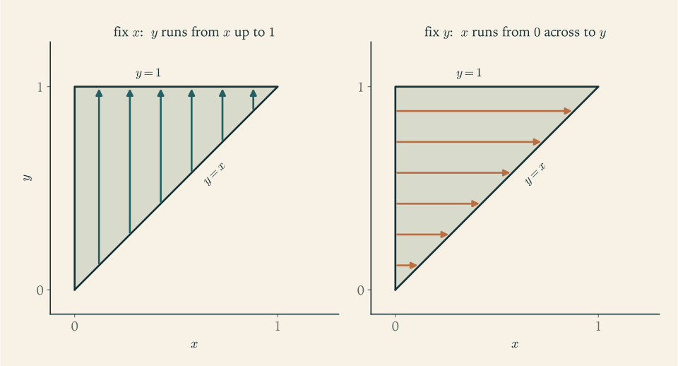
Figure 6.1 shows the two ways of slicing the triangle. Described by horizontal slices, \(y\) runs from \(0\) to \(1\) , and for each \(y\) the variable \(x\) runs from the left edge \(x=0\) to the diagonal \(x=y\) . So, by Theorem 6.4 applied twice,

\[ \int_0^1\!\!\int_x^1e^{y^{2}}\,dy\,dx=\iint_De^{y^{2}}\,dA=\int_0^1\!\!\int_0^ye^{y^{2}}\,dx\,dy=\int_0^1ye^{y^{2}}\,dy=\Bigl[\tfrac12e^{y^{2}}\Bigr]_0^1=\frac{e-1}{2}\approx 0.859 . \]

The inner integration in \(x\) was trivial because the integrand does not involve \(x\) ; it merely produced the length \(y\) of the slice, and that factor \(y\) is exactly what was needed to integrate \(e^{y^{2}}\) .

Common mistake. Reversing the order by exchanging the integral signs and keeping the limits: writing \(\int_0^1\int_x^1f\,dy\,dx\) as \(\int_x^1\int_0^1f\,dx\,dy\) . The result has an outer limit that depends on \(x\) , a variable that has already been integrated away, so it is not a number at all. The limits of an iterated integral are a description of a region, and a different order of integration needs a different description of the same region. Sketch the region, mark a typical slice in the new direction, and read off where it enters and leaves.

6.5 When the two orders disagree

Fubini’s theorem has a hypothesis, continuity on the closed rectangle, and a function that violates it badly enough can have two iterated integrals that both exist and are different.

6.6 Triple integrals

Everything above extends to three variables. For a continuous function \(f\) on a box \(B=[a,b]\times[c,d]\times[p,q]\) , Riemann sums over partitions into small boxes converge to the triple integral \(\iiint_Bf\,dV\) , and Fubini’s theorem equates it with an iterated integral in any of the six possible orders. For a bounded solid \(E\) one extends \(f\) by zero as before. The most common description is as the solid between two graphs over a plane region,

after which the outer double integral over the shadow \(D\) is handled by the methods of Section 6.3. The integral of \(1\) is the volume of \(E\) ; the integral of a density is a mass; averages and centres of mass are defined as in the plane.

Setting up a triple integral is an exercise in seeing a solid. Decide which variable to integrate first, find the two surfaces between which that variable runs, then project the solid onto the plane of the other two variables and describe the shadow.

Exercises

1. Define a Riemann sum for a function on a rectangle and the double integral as a limit of such sums, state Fubini’s theorem with its hypothesis, and name the example of this chapter that shows the hypothesis cannot simply be dropped.

2. Evaluate \(\iint_Rxy^{2}\,dA\) over \(R=[0,2]\times[1,3]\) as an iterated integral in both orders, and explain how the answer could have been written down as a product of two single integrals.

   Answer

   In either order the value is \(\tfrac{52}{3}\) . Since the integrand is a product \(g(x)h(y)\) and the region is a rectangle, the integral is \(\bigl(\int_0^2x\,dx\bigr)\bigl(\int_1^3y^{2}\,dy\bigr)=2\cdot\tfrac{26}{3}\) .

3. For \(f(x,y)=x+y\) on the unit square divided into \(n^{2}\) equal squares, compute the Riemann sum that samples each square at its lower left corner, evaluate it for \(n=2\) , and find its limit as \(n\to\infty\) .

   Answer

   The lower left corner of the square in column \(i\) and row \(j\) is \(((i-1)/n,(j-1)/n)\) , and the sum is \(S_n=(n-1)/n\) . For \(n=2\) it is \(\tfrac12\) , and \(S_n\to 1\) , the value of \(\iint(x+y)\,dA\) . Every \(S_n\) underestimates, because the function is sampled where it is smallest.

4. Evaluate \(\iint_Dxy\,dA\) where \(D\) is the region between the line \(y=x\) and the parabola \(y=x^{2}\) , describing \(D\) as a type I region.

   Solution

   The curves \(y=x\) and \(y=x^{2}\) meet at \(x=0\) and \(x=1\) , and between them the line is above the parabola, since \(x^{2}\le x\) for \(0\le x\le 1\) . So \(D=\{0\le x\le 1,\ x^{2}\le y\le x\}\) , a type I region, and by Theorem 6.4

   \[ \iint_Dxy\,dA=\int_0^1\!\!\int_{x^{2}}^{x}xy\,dy\,dx=\int_0^1x\cdot\tfrac12\bigl(x^{2}-x^{4}\bigr)\,dx=\tfrac12\int_0^1\bigl(x^{3}-x^{5}\bigr)\,dx=\tfrac12\bigl(\tfrac14-\tfrac16\bigr). \]

   The value is \(\tfrac1{24}\) . The inner integration treated \(x\) as a constant and produced a function of \(x\) alone; the inner limits \(x^{2}\) and \(x\) are where a vertical line at position \(x\) enters and leaves the region.

   As a check, the region is also of type II. A horizontal line at height \(y\) between \(0\) and \(1\) enters at the line, \(x=y\) , and leaves at the parabola, \(x=\sqrt y\) , so \(D=\{0\le y\le 1,\ y\le x\le\sqrt y\}\) and \(\int_0^1\int_y^{\sqrt y}xy\,dx\,dy=\int_0^1\tfrac12y(y-y^{2})\,dy=\tfrac12(\tfrac13-\tfrac14)\) , the same number.

5. Sketch the region of integration of \(\displaystyle\int_0^4\!\!\int_{\sqrt x}^{2}\frac{1}{1+y^{3}}\,dy\,dx\) , reverse the order of integration, and evaluate the integral.

   Solution

   The limits say \(0\le x\le 4\) and \(\sqrt x\le y\le 2\) . The region lies above the curve \(y=\sqrt x\) , that is, to the left of the parabola \(x=y^{2}\) , below the line \(y=2\) , and to the right of the \(y\) -axis. Its corners are \((0,0)\) , \((0,2)\) , and \((4,2)\) .

   Slice horizontally. The heights run from \(y=0\) to \(y=2\) , and at height \(y\) the slice runs from the \(y\) -axis, \(x=0\) , to the parabola, \(x=y^{2}\) . Hence

   \[ \int_0^4\!\!\int_{\sqrt x}^{2}\frac{1}{1+y^{3}}\,dy\,dx=\int_0^2\!\!\int_0^{y^{2}}\frac{1}{1+y^{3}}\,dx\,dy=\int_0^2\frac{y^{2}}{1+y^{3}}\,dy . \]

   The inner integration produced the factor \(y^{2}\) , which is, up to the constant \(3\) , the derivative of \(1+y^{3}\) . So the integral is \(\tfrac13\bigl[\ln(1+y^{3})\bigr]_0^2=\tfrac13\ln 9\) , which equals \(\tfrac23\ln 3\approx 0.732\) . In the original order the inner integral \(\int dy/(1+y^{3})\) is possible by partial fractions but long; the reversal avoids it entirely.

6. Evaluate \(\displaystyle\int_0^1\!\!\int_y^1\sin(x^{2})\,dx\,dy\) by reversing the order of integration, and explain why the integral cannot be started in the order given.

   Solution

   In the given order the inner integral is \(\int_y^1\sin(x^{2})\,dx\) , and \(\sin(x^{2})\) has no antiderivative expressible in elementary functions, so the computation cannot begin.

   The limits say \(0\le y\le 1\) and \(y\le x\le 1\) : the triangle with vertices \((0,0)\) , \((1,0)\) , and \((1,1)\) , below the diagonal. Sliced vertically, \(x\) runs from \(0\) to \(1\) and, for each \(x\) , \(y\) runs from the bottom edge \(y=0\) up to the diagonal \(y=x\) . Therefore

   \[ \int_0^1\!\!\int_y^1\sin(x^{2})\,dx\,dy=\int_0^1\!\!\int_0^{x}\sin(x^{2})\,dy\,dx=\int_0^1x\sin(x^{2})\,dx=\Bigl[-\tfrac12\cos(x^{2})\Bigr]_0^1 , \]

   which is \(\frac{1-\cos 1}{2}\approx 0.230\) . As in Example 6.4, integrating first in the variable that the integrand does not contain supplies the factor that makes the remaining integral elementary.

7. Write the area of the region between \(y=x^{2}\) and \(y=x+2\) as a sum of two iterated integrals in the order \(dx\,dy\) , evaluate them, and confirm the value found in Example 6.3.

   Solution

   The region lies between heights \(y=0\) , the vertex of the parabola, and \(y=4\) , the height of the upper intersection point \((2,4)\) . The lower intersection point is \((-1,1)\) .

   For \(0\le y\le 1\) a horizontal line meets only the parabola, entering at \(x=-\sqrt y\) and leaving at \(x=\sqrt y\) . For \(1\le y\le 4\) it enters at the line \(y=x+2\) , that is, at \(x=y-2\) , and leaves at the right branch of the parabola, \(x=\sqrt y\) . So

   \[ \operatorname{area}(D)=\int_0^1\!\!\int_{-\sqrt y}^{\sqrt y}dx\,dy+\int_1^4\!\!\int_{y-2}^{\sqrt y}dx\,dy=\int_0^1 2\sqrt y\,dy+\int_1^4\bigl(\sqrt y-y+2\bigr)\,dy . \]

   The first integral is \(\tfrac43\) . The second is \(\bigl[\tfrac23y^{3/2}-\tfrac12y^{2}+2y\bigr]_1^4=\bigl(\tfrac{16}{3}-8+8\bigr)-\bigl(\tfrac23-\tfrac12+2\bigr)=\tfrac{16}{3}-\tfrac{13}{6}=\tfrac{19}{6}\) . The total is \(\tfrac43+\tfrac{19}{6}=\tfrac{27}{6}=\tfrac92\) , as in Example 6.3. The type I description needed one integral and the type II description two, because the left boundary is given by different formulas below and above \(y=1\) .

8. Find the volume of the solid under the surface \(z=xy\) and above the triangle in the \(xy\) -plane with vertices \((0,0)\) , \((1,0)\) , and \((1,2)\) .

   Hint

   The triangle is \(0\le x\le 1\) , \(0\le y\le 2x\) : its slanted side joins \((0,0)\) to \((1,2)\) . The volume is \(\int_0^1\int_0^{2x}xy\,dy\,dx\) , and the inner integral is \(2x^{3}\) . You should get \(\tfrac12\) .

9. Let \(f\) be continuous on a closed bounded convex region \(D\) of positive area, such as a rectangle or a disc. Prove that there is a point of \(D\) at which \(f\) equals its average value over \(D\) , and explain why the same argument applies to a continuous function on a solid ball in space.

   Solution

   The region \(D\) is closed and bounded and \(f\) is continuous, so by the extreme value theorem \(f\) attains a minimum \(m\) at some point \(\mathbf p\in D\) and a maximum \(M\) at some point \(\mathbf q\in D\) . Since \(m\le f\le M\) on \(D\) , monotonicity and linearity of the integral over \(D\) give

   \[ m\cdot\operatorname{area}(D)\le\iint_Df\,dA\le M\cdot\operatorname{area}(D), \]

   because \(\iint_D1\,dA=\operatorname{area}(D)\) . Dividing by the area, which is positive, the average value \(A=\iint_Df\,dA/\operatorname{area}(D)\) satisfies \(m\le A\le M\) .

   Now join \(\mathbf p\) to \(\mathbf q\) by the segment \(\mathbf r(t)=\mathbf p+t(\mathbf q-\mathbf p)\) , \(0\le t\le 1\) . A set is convex when it contains the segment joining any two of its points, so the segment lies in \(D\) . The function \(g(t)=f(\mathbf r(t))\) is a composition of continuous functions, hence continuous on \([0,1]\) , with \(g(0)=m\) and \(g(1)=M\) . By the intermediate value theorem of single-variable calculus there is \(t_0\in[0,1]\) with \(g(t_0)=A\) . The point \(\mathbf r(t_0)\) belongs to \(D\) , and \(f\) equals its average there.

   The argument used four things: the region is closed and bounded, so that the extreme value theorem applies; it has positive area; it contains the segment joining two of its points; and the integral is monotone. None of them is special to two dimensions. A solid ball is closed, bounded, and convex and has positive volume, and the triple integral is monotone, so a continuous function on a ball equals its average over the ball at some point of the ball. Rectangles, discs, and flat discs in space are covered in the same way.

10. For \(f(x,y)=(x-y)/(x+y)^{3}\) on the square \(0<x\le 1\) , \(0<y\le 1\) , compute both iterated integrals and explain why their disagreement does not contradict Fubini’s theorem.

    Solution

    For fixed \(x>0\) write the numerator as \(x-y=2x-(x+y)\) . Then

    \[ \int_0^1\frac{x-y}{(x+y)^{3}}\,dy=\int_0^1\Bigl(\frac{2x}{(x+y)^{3}}-\frac{1}{(x+y)^{2}}\Bigr)dy=\Bigl[-\frac{x}{(x+y)^{2}}+\frac{1}{x+y}\Bigr]_{y=0}^{y=1}. \]

    At \(y=1\) the bracket is \(-x/(1+x)^{2}+1/(1+x)=1/(1+x)^{2}\) , and at \(y=0\) it is \(-1/x+1/x=0\) . So the inner integral is \(\frac{1}{(1+x)^{2}}\) , and

    \[ \int_0^1\!\!\int_0^1f\,dy\,dx=\int_0^1\frac{dx}{(1+x)^{2}}=\Bigl[-\frac1{1+x}\Bigr]_0^1 , \]

    which is \(\tfrac12\) . Exchanging the names of \(x\) and \(y\) turns \(f\) into \(-f\) , so the same computation gives the other iterated integral \(\int_0^1\int_0^1f\,dx\,dy\) as \(-\tfrac12\) .

    The two iterated integrals exist and differ. Fubini’s theorem is not contradicted because its hypothesis fails: \(f\) is not continuous on the closed square and is unbounded near the origin, where \(f(x,0)=1/x^{2}\) . Theorem 6.2 says nothing about such a function. The disagreement shows that the function is not integrable over the square in the sense of Definition 6.1.

11. A student rewrites \(\displaystyle\int_0^1\!\!\int_0^xf(x,y)\,dy\,dx\) as \(\displaystyle\int_0^x\!\!\int_0^1f(x,y)\,dx\,dy\) . Explain why the second expression cannot be correct whatever \(f\) is, give the correct reversed integral, and verify your answer with \(f(x,y)=y\) .

    Solution

    In the second expression the outer integral has upper limit \(x\) . But \(x\) is the variable of the inner integration; once the inner integral has been evaluated, \(x\) no longer appears, so an outer limit involving \(x\) is meaningless. If one evaluates it formally the “answer” still contains the letter \(x\) , whereas the original integral is a number. No choice of \(f\) can repair that.

    The original limits describe the region \(0\le x\le 1\) , \(0\le y\le x\) : the triangle below the diagonal with vertices \((0,0)\) , \((1,0)\) , \((1,1)\) . Sliced horizontally, \(y\) runs from \(0\) to \(1\) and, for each \(y\) , \(x\) runs from the diagonal \(x=y\) to the right edge \(x=1\) . The correct reversal is

    \[ \int_0^1\int_y^1 f(x,y)\,dx\,dy . \]

    With \(f(x,y)=y\) : the original integral is \(\int_0^1\tfrac12x^{2}\,dx\) , which is \(\tfrac16\) ; the reversed one is \(\int_0^1y(1-y)\,dy=\tfrac12-\tfrac13\) , also \(\tfrac16\) .

12. Evaluate \(\iiint_Ex\,dV\) where \(E\) is the solid given by \(0\le x\le 1\) , \(0\le y\le x\) , \(0\le z\le x+y\) .

    Hint

    Integrate in \(z\) first to get \(x(x+y)\) , then in \(y\) from \(0\) to \(x\) to get \(x^{3}+\tfrac12x^{3}\) . The value is \(\tfrac38\) .

13. The tetrahedron with vertices \((0,0,0)\) , \((1,0,0)\) , \((0,2,0)\) , and \((0,0,3)\) is bounded by the coordinate planes and one further plane. Find that plane, set up the volume as an iterated integral in the order \(dz\,dy\,dx\) and again in the order \(dx\,dy\,dz\) , and evaluate one of them.

    Hint

    The plane through \((1,0,0)\) , \((0,2,0)\) , \((0,0,3)\) is \(x+\tfrac y2+\tfrac z3=1\) . In the order \(dz\,dy\,dx\) the limits are \(0\le z\le 3-3x-\tfrac32y\) , \(0\le y\le 2-2x\) , \(0\le x\le 1\) ; in the order \(dx\,dy\,dz\) they are \(0\le x\le 1-\tfrac y2-\tfrac z3\) , \(0\le y\le 2-\tfrac23z\) , \(0\le z\le 3\) . The volume is \(1\) , one sixth of the product of the three intercepts.

14. A triangular plate occupies \(0\le y\le x\le 1\) and has density \(\rho(x,y)=x\) . Find its mass and its centre of mass.

    Solution

    The plate is the type I region \(0\le x\le 1\) , \(0\le y\le x\) . Its mass is

    \[ M=\iint_Dx\,dA=\int_0^1\!\!\int_0^xx\,dy\,dx=\int_0^1x^{2}\,dx , \]

    which is \(\tfrac13\) . The moments are

    \[ \iint_Dx\cdot x\,dA=\int_0^1x^{3}\,dx=\tfrac14,\qquad\iint_Dy\cdot x\,dA=\int_0^1x\cdot\tfrac12x^{2}\,dx=\tfrac18 . \]

    Dividing by the mass, \(\bar x=\tfrac34\) and \(\bar y=\tfrac38\) : the centre of mass is \((\tfrac34,\tfrac38)\) .

    For comparison, the centroid of the same triangle with constant density is the average of its vertices, \((\tfrac23,\tfrac13)\) . The density \(\rho=x\) is heavier toward the right edge, and the centre of mass has moved to the right accordingly, and slightly upward because the right part of the triangle is also the taller part.

15. Find the average value of the squared distance from the origin, \(x^{2}+y^{2}\) , over the triangle with vertices \((0,0)\) , \((1,0)\) , and \((0,1)\) .

    Answer

    \(\iint(x^{2}+y^{2})\,dA=2\int_0^1x^{2}(1-x)\,dx=\tfrac16\) by symmetry between \(x\) and \(y\) , and the area is \(\tfrac12\) , so the average is \(\tfrac13\) .

16. Describe in words the solid whose volume is given by \(\displaystyle\int_{-1}^{1}\!\!\int_0^{\sqrt{1-x^{2}}}\!\!\int_0^{y}dz\,dy\,dx\) , and compute the volume.

    Answer

    The base is the upper half of the unit disc, \(y\ge 0\) , in the \(xy\) -plane, and the solid lies between the base and the plane \(z=y\) : a wedge cut from a half-cylinder by a plane through the diameter. Its volume is \(\int_{-1}^{1}\tfrac12(1-x^{2})\,dx=\tfrac23\) .

17. Let \(D=\{(x,y):c\le y\le d,\ -h(y)\le x\le h(y)\}\) with \(h\ge 0\) continuous, and let \(f\) be continuous on \(D\) with \(f(-x,y)=-f(x,y)\) . Prove that \(\iint_Df\,dA=0\) , and use this to evaluate \(\iint_D(x^{3}\cos y+2)\,dA\) over the unit disc.

    Solution

    The region is of type II, so by Theorem 6.4

    \[ \iint_Df\,dA=\int_c^d\Bigl(\int_{-h(y)}^{h(y)}f(x,y)\,dx\Bigr)dy . \]

    Fix \(y\) and consider the inner integral. Split it at \(0\) and substitute \(x=-u\) in the part over \([-h(y),0]\) :

    \[ \int_{-h(y)}^{0}f(x,y)\,dx=\int_{0}^{h(y)}f(-u,y)\,du=-\int_0^{h(y)}f(u,y)\,du , \]

    using the hypothesis \(f(-u,y)=-f(u,y)\) . This cancels the part over \([0,h(y)]\) , so the inner integral is \(0\) for every \(y\) , and the outer integral of the zero function is \(0\) .

    The unit disc has this form with \(c=-1\) , \(d=1\) , and \(h(y)=\sqrt{1-y^{2}}\) . The function \(x^{3}\cos y\) is continuous and odd in \(x\) , so its integral over the disc vanishes. By linearity, \(\iint_D(x^{3}\cos y+2)\,dA=0+2\operatorname{area}(D)=2\pi\) . Recognizing an odd integrand over a symmetric region avoids a computation that would otherwise be unpleasant.

18. Find the constants \(a\) and \(b\) that minimize \(E(a,b)=\displaystyle\iint_{[0,1]\times[0,1]}(xy-a-bx)^{2}\,dA\) , confirm with the second derivative test of Chapter 4 that you have found a minimum, and interpret the resulting function \(a+bx\) .

    Solution

    Expand under the integral sign and differentiate, or differentiate first: since \(E\) is a polynomial in \(a\) and \(b\) whose coefficients are integrals, \(E_a=-2\iint(xy-a-bx)\,dA\) and \(E_b=-2\iint x(xy-a-bx)\,dA\) . Over the unit square, \(\iint xy\,dA=\tfrac14\) , \(\iint x\,dA=\tfrac12\) , \(\iint x^{2}y\,dA=\tfrac13\cdot\tfrac12=\tfrac16\) , and \(\iint x^{2}\,dA=\tfrac13\) . The critical point equations are

    \[ \tfrac14-a-\tfrac12b=0,\qquad\tfrac16-\tfrac12a-\tfrac13b=0 . \]

    From the first, \(a=\tfrac14-\tfrac12b\) ; substituting into the second gives \(\tfrac16-\tfrac18+\tfrac14b-\tfrac13b=0\) , so \(\tfrac1{24}=\tfrac1{12}b\) . Hence \(b=\tfrac12\) and \(a=0\) .

    The Hessian of \(E\) is \(\begin{pmatrix}2&1\\ 1&\tfrac23\end{pmatrix}\) , with determinant \(\tfrac43-1=\tfrac13>0\) and positive upper-left entry, so it is positive definite; \(E\) is quadratic, so the critical point is the global minimum. The minimal value is \(\iint(xy-\tfrac12x)^{2}\,dA=\int_0^1x^{2}\,dx\int_0^1(y-\tfrac12)^{2}\,dy=\tfrac13\cdot\tfrac1{12}\) , which is \(\tfrac1{36}\) .

    The best approximation is \(\tfrac12x\) . For each fixed \(x\) this is the average of \(xy\) over \(0\le y\le 1\) : the best way to replace a function of two variables by a function of \(x\) alone, in the least-squares sense, is to average out the other variable.