Pluck a long taut string by pulling a short piece of it sideways and letting go. The bump does not spread and fade as heat would. It divides into two bumps of half the height, which run off in opposite directions at a fixed speed and keep their shape. Someone holding the string ten metres away feels nothing at all until the bump arrives, and then feels exactly the shape that was put in. Three things in this description are foreign to the heat equation: a definite speed, the absence of any smoothing, and the absence of any loss.
The wave equation \(u_{tt}=c^2u_{xx}\) was derived in Section 1.2 from conservation of momentum. In one space dimension it can be solved completely, and the formula makes all three features visible. The chapter then proves the same features a second time by an energy argument that needs no formula, because that argument is the one that survives in higher dimensions and for variable coefficients.
6.1 Two families of travelling waves
Section 1.4 classified the wave equation as hyperbolic with characteristic lines \(x\pm ct=\text{constant}\) , and Exercise 1.16 showed that in the variables \(\xi=x-ct\) , \(\eta=x+ct\) it becomes \(-4c^2w_{\xi\eta}=0\) .
Theorem 6.1 (general solution). A function \(u\in C^2(\mathbb R^2)\) satisfies \(u_{tt}=c^2u_{xx}\) in the \((x,t)\) plane if and only if
for some \(F,G\in C^2(\mathbb R)\) .
Proof. If \(u\) has this form then \(u_{tt}=c^2F''+c^2G''=c^2u_{xx}\) . Conversely let \(w(\xi,\eta)=u(x,t)\) with \(x=\tfrac12(\xi+\eta)\) , \(t=\tfrac{1}{2c}(\eta-\xi)\) ; then \(w\in C^2\) and \(w_{\xi\eta}=0\) . So \(w_\xi\) does not depend on \(\eta\) : \(w_\xi(\xi,\eta)=f(\xi)\) with \(f\in C^1\) . Integrating in \(\xi\) from \(0\) , \(w(\xi,\eta)=F(\xi)+w(0,\eta)\) with \(F(\xi)=\int_0^\xi f\) , which is \(C^2\) , and \(G(\eta)=w(0,\eta)\) is \(C^2\) because \(w\) is.
The term \(F(x-ct)\) is a fixed profile moving to the right at speed \(c\) , and \(G(x+ct)\) is one moving to the left. Every solution is a superposition of one of each. Another way to see the two families is to factor the operator:
If \(u\) solves the wave equation, then \(v=u_t+cu_x\) solves the transport equation \(v_t-cv_x=0\) of Chapter 2, so \(v\) is constant along the lines \(x+ct=\text{constant}\) ; and \(u\) is then obtained from \(v\) by solving a second transport equation along the lines \(x-ct=\text{constant}\) . The wave equation is two transport equations in succession, one for each direction (Exercise 3).
6.2 d’Alembert’s formula
Theorem 6.2 (d’Alembert). Let \(g\in C^2(\mathbb R)\) and \(h\in C^1(\mathbb R)\) . The initial value problem
has exactly one solution \(u\in C^2(\mathbb R^2)\) , given by
Proof. By Theorem 6.1 any solution is \(F(x-ct)+G(x+ct)\) . The initial conditions say \(F+G=g\) and \(-cF'+cG'=h\) . Integrating the second, \(G-F=\tfrac1cH+C\) where \(H(x)=\int_0^xh(s)\,ds\) and \(C\) is a constant. Solving the two linear equations,
Hence \(u=\tfrac12[g(x-ct)+g(x+ct)]+\tfrac{1}{2c}[H(x+ct)-H(x-ct)]\) , the constant cancelling, and this is the stated formula. So there is at most one solution. Conversely these \(F\) and \(G\) are \(C^2\) , because \(g\in C^2\) and \(H\in C^2\) , so the formula defines a \(C^2\) solution, and it satisfies the initial conditions by construction.
The formula has three immediate consequences. First, for \(\lvert t\rvert\le T\) it gives \(\lvert u\rvert\le\sup\lvert g\rvert+T\sup\lvert h\rvert\) , so the solution depends continuously on the data on bounded time intervals, and with existence and uniqueness the problem is well-posed in the sense of Definition 1.4. Second, nothing in the theorem prefers positive \(t\) : the wave equation is solved backward in time as easily as forward, and replacing \(t\) by \(-t\) turns a solution into a solution. Third, \(u\) is exactly as smooth as the data allow, \(C^2\) if \(g\in C^2\) and \(h\in C^1\) , and no smoother. There is no gain of regularity.
Example 6.1: A released bump and a struck string
Released from rest. Let \(g(x)=e^{-x^2}\) and \(h=0\) . Then
At \(t=0\) the two halves coincide and add up to \(g\) . For \(ct\) large compared with the width of the bump they are separate, each a copy of the initial shape at half height.
Struck while flat. Let \(g=0\) and \(h(x)=\cos x\) . Then \(\int_{x-ct}^{x+ct}\cos s\,ds=\sin(x+ct)-\sin(x-ct)=2\cos x\sin(ct)\) , so
Check: \(u_{tt}=-c\cos x\sin(ct)\) and \(c^2u_{xx}=-c\cos x\sin(ct)\) , and \(u(x,0)=0\) , \(u_t(x,0)=\cos x\) . This solution does not appear to travel at all: it is a standing wave, a fixed shape \(\cos x\) whose amplitude oscillates in time. The computation shows what a standing wave is: the sum of two equal travelling waves moving in opposite directions, \(\tfrac{1}{2c}\sin(x+ct)\) and \(-\tfrac{1}{2c}\sin(x-ct)\) .
6.3 Domain of dependence and range of influence
Look at what the formula uses. The value \(u(x_0,t_0)\) , for \(t_0>0\) , depends on \(g\) only at the two points \(x_0\pm ct_0\) and on \(h\) only on the interval between them.
Definition 6.3 (domain of dependence, range of influence). The domain of dependence of the point \((x_0,t_0)\) , \(t_0>0\) , is the interval \([x_0-ct_0,\,x_0+ct_0]\) of the initial line; together with the two characteristic lines through \((x_0,t_0)\) it bounds the characteristic triangle of that point. The range of influence of an interval \([a,b]\) of the initial line is the set of points \((x,t)\) , \(t\ge0\) , whose domain of dependence meets \([a,b]\) , that is, the region \(a-ct\le x\le b+ct\) .
Initial data outside the domain of dependence have no effect on \(u(x_0,t_0)\) . Equivalently, a disturbance initially confined to \([a,b]\) is confined at time \(t\) to \([a-ct,b+ct]\) : its edge moves outward at speed exactly \(c\) , and a point at distance \(d\) from the interval is undisturbed until the time \(d/c\) . This is finite speed of propagation, and \(c\) is that speed.
Example 6.2: Timing a signal
Take \(c=1\) and the tent-shaped displacement \(g(x)=\max(0,1-\lvert x\rvert)\) , supported on \([-1,1]\) , with \(h=0\) . This \(g\) has corners, so it is not \(C^2\) and Theorem 6.2 does not literally apply. We use the formula anyway; Chapter 8 will explain in what sense the result is a solution. The solution is \(u=\tfrac12g(x-t)+\tfrac12g(x+t)\) , two half-height tents.
At the point \(x=0.5\) and time \(t=1\) , \(u=\tfrac12g(-0.5)+\tfrac12g(1.5)=\tfrac12\cdot0.5+0=0.25\) . An observer at \(x=5\) sees nothing while \(t\le4\) , because the nearest point of the support is at distance \(4\) . The right-moving tent then passes: \(u(5,t)=\tfrac12g(5-t)\) rises to its maximum \(0.5\) at \(t=5\) and returns to zero at \(t=6\) , after which the observer is again at rest for ever. The corners of the tent, at its peak and at its two feet, travel with it along characteristic lines and are never smoothed.
Now strike the string instead: \(g=0\) and \(h=1\) on \([-1,1]\) , \(h=0\) elsewhere. The formula gives \(u(x,t)=\tfrac12\) times the length of the part of \([x-t,x+t]\) that lies in \([-1,1]\) . At \(x=5\) this is \(0\) for \(t\le4\) , then \(\tfrac12(t-4)\) for \(4\le t\le6\) , and then \(1\) for all \(t\ge6\) . The signal arrives at the same time as before, but it does not leave: the string is permanently displaced by \(\tfrac{1}{2c}\int h\,ds=1\) .
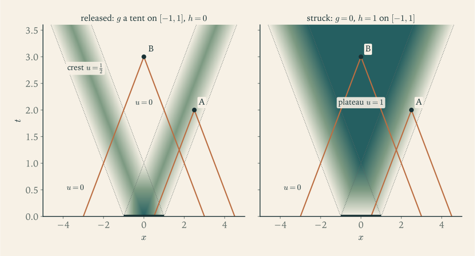
Figure 6.1 shows both solutions, with the characteristic triangles of the points \(A=(2.5,2)\) and \(B=(0,3)\) . In the left panel \(A\) lies in the right-moving strip because one corner of its triangle, at \(x=0.5\) , falls inside the support of \(g\) , giving \(u(A)=\tfrac12g(0.5)=0.25\) . The point \(B\) has the whole support inside the base of its triangle and still has \(u(B)=0\) , because neither corner, at \(x=\pm3\) , touches it. In the right panel that same point has \(u(B)=1\) : the velocity data count along the whole base.
6.4 Energy
For a string with density \(\rho\) and tension \(T\) the kinetic energy per unit length is \(\tfrac12\rho u_t^2\) and the potential energy of stretching is, for small slopes, \(\tfrac12Tu_x^2\) . Dividing by \(\rho\) and using \(c^2=T/\rho\) we define the energy of a solution on \([0,L]\) as
Theorem 6.4 (conservation of energy). Let \(u\in C^2([0,L]\times[0,\infty))\) satisfy \(u_{tt}=c^2u_{xx}\) with either \(u=0\) or \(u_x=0\) at each of the ends \(x=0\) and \(x=L\) for all \(t\) . Then \(E(t)=E(0)\) for all \(t\ge0\) .
Proof. Differentiating under the integral and using the equation,
At an end where \(u=0\) for all \(t\) we have \(u_t=0\) ; at an end where \(u_x=0\) the product vanishes for that reason. So \(E'=0\) .
The quantity \(-c^2u_tu_x\) is the flux of energy in the positive \(x\) -direction, and the computation is the conservation law of Section 1.2 for the energy density \(\tfrac12(u_t^2+c^2u_x^2)\) . A fixed end and a free end both do no work on the string, and the energy stays inside. Compare Theorem 5.7, where the corresponding quantity strictly decreased.
Theorem 6.5 (uniqueness for the vibrating string). The problem \(u_{tt}-c^2u_{xx}=f\) on \(0<x<L\) , \(t>0\) , with prescribed \(u(x,0)\) , \(u_t(x,0)\) and prescribed values of \(u\) at \(x=0\) and \(x=L\) has at most one solution in \(C^2([0,L]\times[0,\infty))\) .
Proof. The difference \(w\) of two solutions satisfies the homogeneous equation with \(w=0\) at both ends and \(w=w_t=0\) at \(t=0\) . Then \(w_x(x,0)=0\) too, so its energy at time zero is zero, and by Theorem 6.4 it is zero for all time. Hence \(w_t=w_x=0\) everywhere, \(w\) is constant, and the constant is its initial value, zero.
The same computation, carried out on a shrinking interval, proves finite propagation speed without any solution formula.
Theorem 6.6 (energy in a characteristic triangle). Let \(u\) be a \(C^2\) solution of \(u_{tt}=c^2u_{xx}\) in a region containing the characteristic triangle of \((x_0,t_0)\) , and for \(0\le t\le t_0\) put
Then \(e\) is nonincreasing. In particular, if \(u(x,0)=u_t(x,0)=0\) on the base \([x_0-ct_0,x_0+ct_0]\) , then \(u=0\) throughout the triangle.
Proof. The endpoints \(x_\pm(t)=x_0\pm c(t_0-t)\) move inward at speed \(c\) . By the Leibniz rule and the computation in the proof of Theorem 6.4,
Collecting the terms at each endpoint,
If the data vanish on the base then \(u_x(x,0)=0\) there as well, so \(e(0)=0\) , and since \(0\le e(t)\le e(0)\) we get \(e=0\) . Thus \(u_t=u_x=0\) in the triangle, \(u\) is constant there, and the constant is zero.
The theorem says that energy can leave the shrinking interval through its ends but cannot enter: the ends move inward at the wave speed, and nothing travels faster. Applied to the difference of two solutions it shows directly that the solution in the triangle is determined by the data on its base, which is the content of Definition 6.3, now with a proof that does not depend on d’Alembert’s formula.
Example 6.3: Energy sloshing in a standing wave
On \(0\le x\le1\) the function \(u=\sin(\pi x)\cos(\pi ct)\) solves the wave equation and vanishes at both ends. Its kinetic and potential parts are
using \(\int_0^1\sin^2(\pi x)\,dx=\int_0^1\cos^2(\pi x)\,dx=\tfrac12\) . Their sum is \(E=\pi^2c^2/4\) at every instant. At \(t=0\) the string is at rest in its most stretched shape and the energy is all potential. A quarter period later, at \(ct=\tfrac12\) , the string is flat and moving fastest, and the energy is all kinetic. The total never changes.
6.5 Reflection at a boundary
A string that occupies \(x\ge0\) and is held fixed at \(x=0\) satisfies \(u(0,t)=0\) . An odd function vanishes at the origin, and d’Alembert’s formula applied to odd data produces a solution that is odd in \(x\) at every time. So extend \(g\) and \(h\) to odd functions on the line and apply Theorem 6.2. That theorem needs the extended \(g\) to be \(C^2\) and the extended \(h\) to be \(C^1\) , which holds exactly when \(g(0)=g''(0)=0\) and \(h(0)=0\) . These compatibility conditions say that the data agree with the boundary condition, and with the equation, at the corner where the initial line meets the boundary. When they fail the formula below still makes sense, and it is a solution in the distributional sense of Chapter 8. For \(x\ge ct\) the interval \([x-ct,x+ct]\) lies in the half-line and nothing changes. For \(0\le x<ct\) the point \(x-ct\) is negative; using the oddness, \(g(x-ct)=-g(ct-x)\) and the integral of \(h\) over \([x-ct,ct-x]\) cancels, leaving
The left-moving wave has reached the wall and come back as a right-moving wave with its sign reversed. For a free end, \(u_x(0,t)=0\) , the same argument with an even extension gives a reflection without change of sign; the compatibility conditions are then \(g'(0)=0\) and \(h'(0)=0\) . For a string of finite length \(L\) fixed at both ends, extend the data to be odd about \(x=0\) and about \(x=L\) , which makes them periodic with period \(2L\) and requires the conditions \(g=g''=0\) and \(h=0\) at both ends; the waves reflect back and forth, and the motion repeats itself exactly after the time \(2L/c\) (Exercise 13). This construction is the image method of Section 4.5 in a new setting.
Example 6.4: A pulse meets a fixed end
On the half-line \(x\ge0\) with \(u(0,t)=0\) and \(c=1\) , release from rest the tent \(g(x)=\max(0,1-\lvert x-3\rvert)\) , centred at \(x=3\) . It splits into two half-height tents. The right-moving one is centred at \(x=3+t\) . The left-moving one is centred at \(x=3-t\) , reaches the wall at \(t=3\) , and reflects.
At \(t=4\) and \(x=7\) we have \(x>ct\) , and \(u=\tfrac12[g(11)+g(3)]=\tfrac12\) : the peak of the right-moving tent. At \(t=4\) and \(x=1\) we have \(x<ct\) , so the reflection formula applies: \(u=\tfrac12[g(5)-g(3)]=\tfrac12[0-1]=-\tfrac12\) . The reflected pulse is centred at \(x=1\) , moving right, and upside down. During the reflection, at \(t=3\) , the incoming and the inverted outgoing pulse overlap near the wall and cancel exactly at \(x=0\) , which is how the boundary condition is kept.
6.6 Sources, resonance, and higher dimensions
Theorem 6.7 (Duhamel’s formula for the wave equation). Let \(f\) and \(f_x\) be continuous on \(\mathbb R\times[0,\infty)\) . Then
is a \(C^2\) solution of \(u_{tt}-c^2u_{xx}=f\) for \(t>0\) with \(u(x,0)=u_t(x,0)=0\) .
Proof. Differentiating in \(t\) , the contribution of the upper limit \(s=t\) is the inner integral over an interval of length zero, so
Differentiating again, the upper limit now contributes \(\tfrac12[f(x,t)+f(x,t)]=f(x,t)\) , and
In \(x\) we get \(u_x=\tfrac{1}{2c}\int_0^t[f(x+c(t-s),s)-f(x-c(t-s),s)]\,ds\) and \(u_{xx}=\tfrac{1}{2c}\int_0^t[f_x(x+c(t-s),s)-f_x(x-c(t-s),s)]\,ds\) . Hence \(u_{tt}-c^2u_{xx}=f\) . The initial values vanish because the integrals are over an interval of length zero when \(t=0\) .
The region of integration is the whole characteristic triangle of \((x,t)\) : a source acts on a point exactly when it lies in that point’s past, within reach at speed \(c\) . The inner integral is d’Alembert’s formula for a string struck at time \(s\) with velocity \(f(\cdot,s)\) .
Example 6.5: A forced string and resonance
Let \(c=1\) and \(f(x,t)=\sin x\) . The inner integral is \(\cos(x-(t-s))-\cos(x+(t-s))=2\sin x\sin(t-s)\) , so
Check: \(u_{tt}=\cos t\sin x\) and \(-u_{xx}=(1-\cos t)\sin x\) , which add up to \(\sin x\) . Under the same steady source the heat equation settled down to a steady state (Example 5.5). The string does not settle: it oscillates for ever about the equilibrium shape \(\sin x\) , because nothing dissipates the energy of the initial mismatch.
Now let the source oscillate at the natural frequency of the mode, \(f(x,t)=\sin x\cos t\) . The solution with zero initial values is
as one verifies: \(u_{tt}=(\cos t-\tfrac12t\sin t)\sin x\) and \(u_{xx}=-\tfrac12t\sin t\sin x\) , so \(u_{tt}-u_{xx}=\cos t\sin x\) . The amplitude grows linearly without bound. This is resonance, and it is possible only because the wave equation has no damping.
In more space dimensions the wave equation \(u_{tt}=c^2\Delta u\) keeps the properties proved by energy: the energy \(\tfrac12\int(u_t^2+c^2\lvert\nabla u\rvert^2)\,dx\) is conserved, and the argument of Theorem 6.6, carried out on a shrinking ball, shows that the solution at \((x_0,t_0)\) depends only on the data in the ball of radius \(ct_0\) about \(x_0\) . The explicit formulas, Kirchhoff’s in three dimensions and Poisson’s in two, belong to a more advanced course. They reveal a difference that the energy method cannot see: in three dimensions the solution depends only on the data on the sphere of radius \(ct_0\) , so a sharp signal is heard sharply and then is over, while in two dimensions, as in one dimension for velocity data, it depends on the whole disc and the signal leaves a tail.
Common mistake. Carrying intuition from the heat equation over to waves. The wave equation has no maximum principle: the struck string of Example 6.1 starts from \(u=0\) and reaches the amplitude \(1/c\) , so the solution is not bounded by the size of its initial displacement. It does not smooth: a corner in the data is still a corner at every later time. And the factor in front of the velocity term is \(\tfrac{1}{2c}\) with limits \(x\pm ct\) ; a quick test of any remembered version of the formula is to differentiate it in \(t\) at \(t=0\) and see whether \(h(x)\) comes out. On a bounded string the formula must not be applied to the data as given, since it knows nothing of the ends; extend the data first by the reflection rule that matches the boundary condition.
The three model equations have now each been solved in a setting with no boundary, or the simplest one. For a finite rod or string with general data the reflections pile up, and a different organisation of the solution becomes natural: instead of following pulses back and forth, decompose the motion into standing waves like that of Example 6.3. Which standing waves are possible on a given interval, and can every initial shape be built from them?
Exercises
-
For \(c=2\) , \(g(x)=1/(1+x^2)\) , and \(h=0\) , write the solution of the initial value problem and evaluate \(u(0,1)\) and \(u(2,1)\) .
Answer
\(u(x,t)=\tfrac12\bigl[g(x+2t)+g(x-2t)\bigr]\) with \(g(s)=1/(1+s^2)\) . Then \(u(0,1)=\tfrac12[g(2)+g(-2)]=\tfrac15\) and \(u(2,1)=\tfrac12[g(4)+g(0)]=\tfrac12\bigl(\tfrac1{17}+1\bigr)=\tfrac{9}{17}\) .
-
Solve the initial value problem with \(g=0\) and \(h(x)=xe^{-x^2}\) , and verify the initial conditions and the equation directly.
Answer
\(\int_{x-ct}^{x+ct}se^{-s^2}ds=\tfrac12\bigl[e^{-(x-ct)^2}-e^{-(x+ct)^2}\bigr]\) , so \(u(x,t)=\dfrac{1}{4c}\bigl[e^{-(x-ct)^2}-e^{-(x+ct)^2}\bigr]\) . At \(t=0\) the two terms cancel, and \(u_t(x,0)=\tfrac{1}{4c}\bigl[2cxe^{-x^2}+2cxe^{-x^2}\bigr]=xe^{-x^2}\) . Each term is a function of \(x-ct\) or \(x+ct\) , so the equation holds by Theorem 6.1.
-
Let \(u\in C^2\) solve \(u_{tt}=c^2u_{xx}\) with \(u(x,0)=g(x)\) and \(u_t(x,0)=h(x)\) . Show that \(v=u_t+cu_x\) satisfies \(v_t-cv_x=0\) and find \(v\) from its initial values using Theorem 2.1; then solve \(u_t+cu_x=v\) with the source formula of Section 2.1 and recover d’Alembert’s formula.
Solution
The first transport equation. Since \(u\in C^2\) , \(v=u_t+cu_x\) is \(C^1\) and \(v_t-cv_x=u_{tt}+cu_{xt}-cu_{tx}-c^2u_{xx}=u_{tt}-c^2u_{xx}=0\) . At \(t=0\) , \(v(x,0)=h(x)+cg'(x)\) . By Theorem 2.1 with speed \(-c\) , \(v(x,t)=(h+cg')(x+ct)\) .
The second. Now \(u_t+cu_x=v\) with \(u(x,0)=g(x)\) . The source formula of Section 2.1 gives
\[ u(x,t)=g(x-ct)+\int_0^tv\bigl(x-c(t-s),s\bigr)\,ds=g(x-ct)+\int_0^t(h+cg')\bigl(x-ct+2cs\bigr)\,ds . \]Substitute \(y=x-ct+2cs\) , so \(ds=dy/(2c)\) and \(y\) runs from \(x-ct\) to \(x+ct\) :
\[ u(x,t)=g(x-ct)+\frac{1}{2c}\int_{x-ct}^{x+ct}h(y)\,dy+\frac12\int_{x-ct}^{x+ct}g'(y)\,dy . \]The last integral is \(\tfrac12[g(x+ct)-g(x-ct)]\) , and adding it to \(g(x-ct)\) gives \(\tfrac12[g(x+ct)+g(x-ct)]\) . This is d’Alembert’s formula. The derivation shows the two transport steps explicitly: \(v\) carries the combination \(h+cg'\) leftward, and \(u\) accumulates it while moving rightward.
-
For the tent \(g(x)=\max(0,1-\lvert x\rvert)\) with \(h=0\) and \(c=1\) , compute \(u(0,\tfrac12)\) , \(u(0,1)\) , \(u(1,1)\) , and \(u(\tfrac12,\tfrac12)\) , and describe the shape of \(u(\cdot,t)\) for \(t=\tfrac12\) and for \(t\ge1\) .
Answer
\(u(0,\tfrac12)=\tfrac12[g(\tfrac12)+g(-\tfrac12)]=\tfrac12\) ; \(u(0,1)=\tfrac12[g(1)+g(-1)]=0\) ; \(u(1,1)=\tfrac12[g(2)+g(0)]=\tfrac12\) ; \(u(\tfrac12,\tfrac12)=\tfrac12[g(1)+g(0)]=\tfrac12\) . At \(t=\tfrac12\) the two half-tents, centred at \(\pm\tfrac12\) , overlap and add up to a trapezoid with a flat top of height \(\tfrac12\) on \([-\tfrac12,\tfrac12]\) and feet at \(\pm\tfrac32\) . For \(t\ge1\) they are disjoint: two tents of height \(\tfrac12\) centred at \(\pm t\) .
-
For \(g=0\) and \(h=1\) on \([-1,1]\) , \(h=0\) elsewhere, with general \(c\) , find \(u(x,t)\) for all \(x\) and \(t>0\) by cases, and show that for each fixed \(x\) the solution equals \(\tfrac{1}{2c}\int h\,ds\) for all sufficiently large \(t\) .
Hint
\(u(x,t)=\tfrac{1}{2c}\) times the length of \([x-ct,x+ct]\cap[-1,1]\) . Distinguish whether each of \(x\pm ct\) lies left of, inside, or right of \([-1,1]\) . Once \(ct\ge\lvert x\rvert+1\) the interval \([x-ct,x+ct]\) contains \([-1,1]\) and \(u=\tfrac{1}{2c}\cdot2=\tfrac1c\) .
-
With \(c=2\) , find the domain of dependence of the point \((x,t)=(3,2)\) , and the set of points at time \(t=2\) that can be influenced by initial data supported in \([0,1]\) . If the data vanish outside \([0,1]\) , at what time does a disturbance first reach \(x=11\) ?
Answer
The domain of dependence of \((3,2)\) is \([3-4,3+4]=[-1,7]\) . Data in \([0,1]\) influence, at \(t=2\) , the points of \([0-4,1+4]=[-4,5]\) . The point \(x=11\) is at distance \(10\) from the support, so it is first reached at \(t=10/2=5\) .
-
For the solution \(u=\tfrac12e^{-(x-ct)^2}+\tfrac12e^{-(x+ct)^2}\) of Example 6.1, compute the energy \(\tfrac12\int_{-\infty}^{\infty}(u_t^2+c^2u_x^2)\,dx\) at \(t=0\) , show that it is the same for all \(t\) , and find the limits of the kinetic and potential parts as \(t\to\infty\) .
Solution
At \(t=0\) the velocity \(u_t\) vanishes, because the data were released from rest, and \(u_x=g'(x)=-2xe^{-x^2}\) . So
\[ E(0)=\frac{c^2}{2}\int_{-\infty}^{\infty}4x^2e^{-2x^2}\,dx=2c^2\cdot\frac{\sqrt\pi}{4\sqrt2}=\frac{c^2}{2}\sqrt{\frac{\pi}{2}}\approx0.627\,c^2 , \]using \(\int x^2e^{-ax^2}dx=\tfrac{\sqrt\pi}{2}a^{-3/2}\) with \(a=2\) .
For general \(t\) write \(u=F(x-ct)+F(x+ct)\) with \(F=\tfrac12g\) . Then \(u_t=-cF'(x-ct)+cF'(x+ct)\) and \(cu_x=cF'(x-ct)+cF'(x+ct)\) , so
\[ u_t^2+c^2u_x^2=2c^2F'(x-ct)^2+2c^2F'(x+ct)^2 , \]the cross terms cancelling. Integrating over the line, each term gives \(2c^2\int F'^2=\tfrac12c^2\int g'^2\) , independent of \(t\) ; so \(E(t)=\tfrac12c^2\int g'^2dx=E(0)\) .
The kinetic part is \(\tfrac12\int u_t^2dx=c^2\int F'^2\,dx-c^2\int F'(x-ct)F'(x+ct)\,dx\) , and the potential part is the same with a plus sign. As \(t\to\infty\) the two factors in the cross integral are concentrated a distance \(2ct\) apart and the integral tends to zero. Hence both parts tend to \(c^2\int F'^2dx=\tfrac12E\) : the energy is eventually shared equally, each travelling pulse carrying equal kinetic and potential energy.
-
Prove that the energy \(\tfrac12\int_{-\infty}^{\infty}(u_t^2+c^2u_x^2)\,dx\) of a \(C^2\) solution on the whole line is constant in time when the initial data vanish outside a bounded interval. Where is finite propagation speed used?
Hint
Compute \(E'(t)\) as in Theorem 6.4 on an interval \([-R,R]\) ; the boundary term is \(c^2[u_tu_x]_{-R}^{R}\) . By finite propagation speed the solution vanishes outside \([a-ct,b+ct]\) , so for \(R\) large, depending on the time interval considered, the boundary term is zero and the integral over \([-R,R]\) is the integral over the line.
-
Prove that the problem \(u_{tt}-c^2u_{xx}=f\) on \(0<x<L\) with prescribed initial data and prescribed \(u_x(0,t)\) and \(u(L,t)\) has at most one \(C^2\) solution.
Solution
Let \(w\) be the difference of two \(C^2\) solutions. Then \(w_{tt}=c^2w_{xx}\) , \(w(x,0)=w_t(x,0)=0\) , \(w_x(0,t)=0\) , and \(w(L,t)=0\) . The last condition gives \(w_t(L,t)=0\) for all \(t\) . With \(E(t)=\tfrac12\int_0^L(w_t^2+c^2w_x^2)\,dx\) , the computation in Theorem 6.4 gives
\[ E'(t)=c^2\bigl[w_tw_x\bigr]_0^L=c^2\,w_t(L,t)\,w_x(L,t)-c^2\,w_t(0,t)\,w_x(0,t)=0 , \]the first product vanishing because \(w_t(L,t)=0\) and the second because \(w_x(0,t)=0\) . At \(t=0\) we have \(w_t=0\) and, differentiating \(w(x,0)=0\) in \(x\) , \(w_x=0\) ; so \(E(0)=0\) and therefore \(E(t)=0\) for all \(t\) . The integrand is continuous and nonnegative, hence \(w_t=w_x=0\) on \([0,L]\times[0,\infty)\) , so \(w\) is constant, equal to its initial value \(0\) . A mixed pair of boundary conditions, one free end and one fixed, is handled by exactly the same identity as two of the same kind.
-
For the damped string \(u_{tt}+2\gamma u_t=c^2u_{xx}\) with \(\gamma>0\) and fixed ends, show that \(E'(t)=-2\gamma\int_0^Lu_t^2\,dx\) , and explain what this says physically.
Answer
\(E'(t)=\int_0^L(u_tu_{tt}+c^2u_xu_{xt})\,dx=\int_0^Lu_t(c^2u_{xx}-2\gamma u_t)\,dx+c^2\int_0^Lu_xu_{xt}\,dx=c^2[u_tu_x]_0^L-2\gamma\int_0^Lu_t^2dx\) , and the boundary term vanishes. Friction proportional to velocity removes energy at a rate proportional to the kinetic energy; the energy decreases whenever the string is moving.
-
A student solves the string with fixed ends at \(x=0\) and \(x=1\) , initial shape \(g(x)=\sin(\pi x)\) and \(h=0\) , by applying d’Alembert’s formula with \(g\) set to zero outside \([0,1]\) . Show that the result violates the boundary condition at \(x=0\) for small positive \(t\) , explain the error, and give the correct solution.
Solution
With \(g\) extended by zero, d’Alembert’s formula gives \(\tilde u(x,t)=\tfrac12[\tilde g(x+ct)+\tilde g(x-ct)]\) . At \(x=0\) and \(0<ct<1\) this is \(\tfrac12[\sin(\pi ct)+0]=\tfrac12\sin(\pi ct)\ne0\) . The end that should be fixed moves.
The error is that Theorem 6.2 solves the problem on the whole line, where there are no ends; the zero extension corresponds to an infinite string that happens to be flat outside \([0,1]\) , and the left-moving half of the initial shape simply runs out through \(x=0\) . To enforce \(u(0,t)=u(1,t)=0\) the data must be extended oddly about both ends, hence \(2\) -periodically, as in Section 6.5. The odd \(2\) -periodic extension of \(\sin(\pi x)\) from \([0,1]\) is \(\sin(\pi x)\) itself, on the whole line. So the correct solution is
\[ u(x,t)=\tfrac12\bigl[\sin(\pi(x+ct))+\sin(\pi(x-ct))\bigr]=\sin(\pi x)\cos(\pi ct), \]the standing wave of Example 6.3. It vanishes at \(x=0\) and \(x=1\) for all \(t\) , has \(u(x,0)=\sin(\pi x)\) and \(u_t(x,0)=0\) , and by Theorem 6.5 it is the only solution.
-
Redo Example 6.4 for a free end, \(u_x(0,t)=0\) : write the formula for \(0\le x<ct\) from the even extension and evaluate \(u(1,4)\) and \(u(0,3)\) .
Answer
For \(0\le x<ct\) the even extension gives \(u(x,t)=\tfrac12[g(ct+x)+g(ct-x)]+\tfrac{1}{2c}\bigl[\int_0^{ct+x}h\,ds+\int_0^{ct-x}h\,ds\bigr]\) . With the data of Example 6.4, \(u(1,4)=\tfrac12[g(5)+g(3)]=+\tfrac12\) : the reflected pulse is upright. And \(u(0,3)=\tfrac12[g(3)+g(3)]=1\) : at the moment of reflection the free end rises to twice the height of the incoming pulse.
-
For a string on \([0,L]\) with fixed ends, let the data be extended as in Section 6.5. Prove from d’Alembert’s formula that \(u(x,t+2L/c)=u(x,t)\) and that \(u(x,t+L/c)=-u(L-x,t)\) , and describe the second identity in words.
Solution
The extended data \(g\) and \(h\) are odd and \(2L\) -periodic. Period. Replacing \(t\) by \(t+2L/c\) changes \(x\pm ct\) to \(x\pm ct\pm2L\) . The values of \(g\) are unchanged by periodicity. The integral of \(h\) over \([x-ct-2L,\,x+ct+2L]\) exceeds that over \([x-ct,x+ct]\) by the integrals over two intervals of length \(2L\) , each a full period of an odd periodic function, hence zero. So \(u(x,t+2L/c)=u(x,t)\) .
Half period. For an odd \(2L\) -periodic function, \(g(L+y)=g(y-L)=-g(L-y)\) . Hence \(g(x+ct+L)=-g\bigl((L-x)-ct\bigr)\) and \(g(x-ct-L)=-g\bigl((L-x)+ct\bigr)\) , so the displacement part of \(u(x,t+L/c)\) is \(-\tfrac12\bigl[g((L-x)-ct)+g((L-x)+ct)\bigr]\) . For the velocity part substitute \(s=L+y\) , use \(h(L+y)=-h(L-y)\) , and then put \(z=L-y\) :
\[ \int_{x-ct-L}^{x+ct+L}h(s)\,ds=-\int_{(L-x)-ct}^{(L-x)+ct+2L}h(z)\,dz=-\int_{(L-x)-ct}^{(L-x)+ct}h(z)\,dz , \]the extra piece being an integral over a full period. Together, \(u(x,t+L/c)=-u(L-x,t)\) .
In words: after half a period the string has the shape it had before, turned upside down and reflected left to right. A pulse that started near the left end is, half a period later, an inverted pulse near the right end.
-
Solve \(u_{tt}-u_{xx}=\sin x\cos(\omega t)\) on the line with zero initial values for \(\omega\ne1\) by looking for \(u=T(t)\sin x\) , and show that as \(\omega\to1\) the solution tends to the resonant solution of Example 6.5.
Solution
With \(u=T(t)\sin x\) we have \(u_{tt}-u_{xx}=(T''+T)\sin x\) , so \(T''+T=\cos(\omega t)\) with \(T(0)=T'(0)=0\) . For \(\omega\ne1\) a particular solution is \(\cos(\omega t)/(1-\omega^2)\) ; adding the solution of the homogeneous equation that fixes the initial values,
\[ T(t)=\frac{\cos(\omega t)-\cos t}{1-\omega^2},\qquad u(x,t)=\frac{\cos(\omega t)-\cos t}{1-\omega^2}\,\sin x . \]Check: \(T''+T=\dfrac{(1-\omega^2)\cos(\omega t)}{1-\omega^2}\) , \(T(0)=0\) , and \(T'(0)=0\) . This is bounded for each fixed \(\omega\ne1\) , with amplitude at most \(2/\lvert1-\omega^2\rvert\) , which is large when \(\omega\) is close to \(1\) .
As \(\omega\to1\) both numerator and denominator tend to zero. Differentiating each with respect to \(\omega\) at \(\omega=1\) gives \(-t\sin t\) and \(-2\) , so \(T(t)\to\tfrac12t\sin t\) , the resonant solution of Example 6.5. Near resonance the solution is a beat: by the sum-to-product formula \(T=\dfrac{2}{1-\omega^2}\sin\!\bigl(\tfrac{(1-\omega)t}{2}\bigr)\sin\!\bigl(\tfrac{(1+\omega)t}{2}\bigr)\) , a fast oscillation inside a slow envelope whose first rise is the linear growth.
-
For each property decide whether it holds for the heat equation, for the wave equation, for both, or for neither, and justify each entry with a theorem or example from Chapters 5 and 6: (a) finite speed of propagation; (b) instantaneous smoothing; (c) a maximum principle; (d) a quantity \(E(t)\) that is conserved; (e) well-posedness backward in time; (f) uniqueness for the initial-boundary value problem on a finite interval.
Answer
(a) Wave only: Definition 6.3 and Theorem 6.6; the heat kernel is positive everywhere (Section 5.2). (b) Heat only: Theorem 5.3(a); by Theorem 6.2 a wave is exactly as smooth as its data. (c) Heat only: Theorem 5.4; the struck string of Example 6.1 starts at zero and reaches amplitude \(1/c\) . (d) Wave only: Theorem 6.4; for the heat equation the quantity of Theorem 5.7 strictly decreases unless the solution is zero. (e) Wave only: Theorem 6.2 holds for all real \(t\) ; for the heat equation see Exercises 1.9 and 5.14. (f) Both: Theorems 5.5 and 6.5.
-
Use Theorem 6.6 to prove, without d’Alembert’s formula, that two \(C^2\) solutions of \(u_{tt}-c^2u_{xx}=f\) on \(\mathbb R\times[0,\infty)\) with the same initial data are equal.
Solution
Let \(u_1,u_2\) be \(C^2\) solutions with the same \(f\) and the same initial data, and put \(w=u_1-u_2\) . Then \(w_{tt}=c^2w_{xx}\) for \(t\ge0\) and \(w(x,0)=w_t(x,0)=0\) for all \(x\) . Fix any point \((x_0,t_0)\) with \(t_0>0\) . Its characteristic triangle lies in the region where \(w\) is a \(C^2\) solution, and the data of \(w\) vanish on the base \([x_0-ct_0,x_0+ct_0]\) . By Theorem 6.6, \(w=0\) throughout the triangle, in particular \(w(x_0,t_0)=0\) . Since the point was arbitrary, \(u_1=u_2\) .
The argument never used a formula for the solution, only the energy inequality \(e'(t)\le0\) , and it proves more than was asked: if two sets of data agree merely on the interval \([x_0-ct_0,x_0+ct_0]\) , the corresponding solutions agree in the triangle above it. That is the precise statement of “domain of dependence”, and it holds, with the same proof, for equations where no analogue of d’Alembert’s formula exists.
-
For the Klein–Gordon equation \(u_{tt}-c^2u_{xx}+m^2u=0\) with fixed ends on \([0,L]\) , find a conserved energy, and find the relation between \(\omega\) and \(\xi\) for which \(e^{i(\xi x-\omega t)}\) is a solution on the line. Do waves of different wave numbers travel at the same speed?
Answer
\(E(t)=\tfrac12\int_0^L(u_t^2+c^2u_x^2+m^2u^2)\,dx\) is conserved: the extra term contributes \(\int m^2uu_t\,dx\) to \(E'\) , which cancels the \(-m^2u\) in \(u_{tt}\) . On the line, \(\omega^2=c^2\xi^2+m^2\) . The speed \(\omega/\xi=\sqrt{c^2+m^2/\xi^2}\) depends on \(\xi\) , so different wave numbers travel at different speeds and a pulse changes shape: the equation is dispersive.