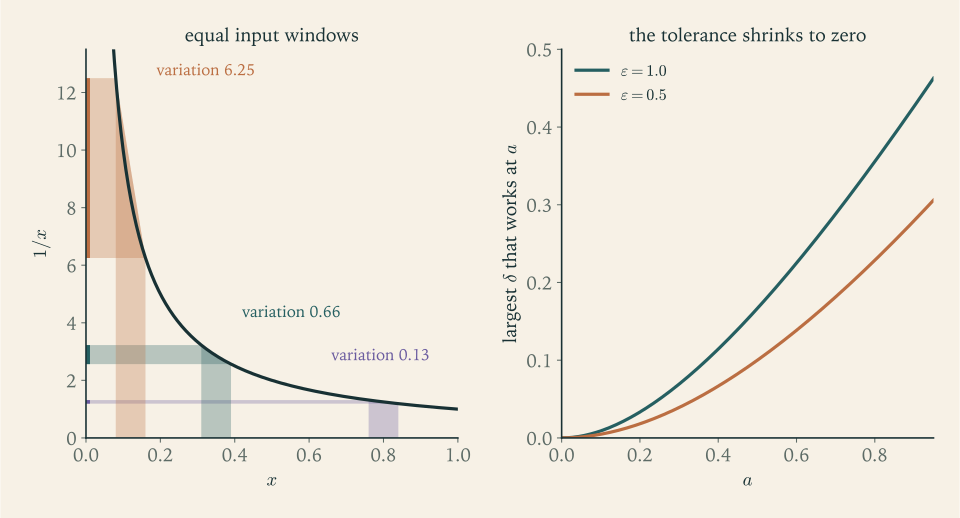
The function \(1/x\) is continuous at every point of the interval \((0,1)\) , and it misbehaves there in three ways. It is unbounded. It has no largest value and no smallest value. And the tolerance it permits shrinks without limit: to keep \(1/x\) within \(1\) of its value at \(a\) , the point \(x\) must stay within about \(a^2\) of \(a\) , which is tiny when \(a\) is near \(0\) . On the closed interval \([\tfrac1{10},1]\) all three problems disappear.

Continuity is a local property; it says something about each point separately. Boundedness, attained extremes, and a single tolerance that works everywhere are global properties. This chapter defines continuity for maps between metric spaces, and then proves that on a compact domain the local property forces the global ones. It also proves the other great theorem about continuous functions on an interval, that they cannot skip values, which depends not on compactness but on the completeness of \(\mathbb R\) .

5.1 Continuity at a point

For a real function defined on a set \(D\subseteq\mathbb R\) , the space \(X\) is \(D\) with the usual distance, and the condition reads: \(\lvert f(x)-f(a)\rvert<\varepsilon\) for all \(x\in D\) with \(\lvert x-a\rvert<\delta\) . Only points of the domain are tested. In terms of balls, the definition says \(f\bigl(B(a,\delta)\bigr)\subseteq B\bigl(f(a),\varepsilon\bigr)\) . The number \(\delta\) may depend on \(\varepsilon\) and on the point \(a\) . It may not depend on \(x\) .

The related notion of a limit ignores the value at the point. If \(a\) is a limit point of \(D\) , we write \(\lim_{x\to a}f(x)=L\) if for every \(\varepsilon>0\) there is \(\delta>0\) with \(d_Y(f(x),L)<\varepsilon\) whenever \(x\in D\) and \(0<d_X(x,a)<\delta\) . Comparing the definitions: at a limit point \(a\in D\) , \(f\) is continuous exactly when \(\lim_{x\to a}f(x)=f(a)\) ; at an isolated point of \(D\) every function is continuous, because for small \(\delta\) the only point tested is \(a\) itself.

5.2 Continuity and open sets

Continuity on a whole space has a formulation with no \(\varepsilon\) and no points at all. For \(f:X\to Y\) and \(V\subseteq Y\) , the preimage is \(f^{-1}(V)=\{x\in X:f(x)\in V\}\) .

Since \(f^{-1}(Y\setminus V)=X\setminus f^{-1}(V)\) , the theorem holds equally with “closed” in place of “open”. It is a quick source of open and closed sets: for continuous \(f:X\to\mathbb R\) the set \(\{x:f(x)>0\}\) is open, as the preimage of \((0,\infty)\) , and \(\{x:f(x)=0\}\) is closed, as the preimage of \(\{0\}\) .

The theorem is about preimages. Images behave worse. The continuous function \(x^2\) maps the open interval \((-1,1)\) onto \([0,1)\) , which is not open. The continuous function \(1/(1+x^2)\) maps the closed set \(\mathbb R\) onto \((0,1]\) , which is not closed. What continuous images do preserve is compactness.

5.3 Continuous functions on compact sets

Compactness of a set \(K\) in a metric space \(X\) does not depend on the ambient space: condition (b) of Theorem 4.17 mentions only sequences in \(K\) and limits in \(K\) . So we may speak of a compact metric space \(K\) and of continuous functions defined only on \(K\) .

In particular, by the Heine–Borel theorem, a continuous real function on a closed bounded interval \([a,b]\) , or on any closed bounded subset of \(\mathbb R^n\) , attains a maximum and a minimum. This is the existence theorem behind every optimisation problem in calculus.

5.4 The Intermediate Value Theorem

The structure is that of Theorem 1.11: take the supremum of the set of points that have not yet reached the target, and show that the supremum can be neither short of the target nor past it. Completeness enters through the supremum, and the theorem fails over \(\mathbb Q\) , as the chapter opening of Chapter 1 showed with \(x^2-2\) .

Call a set \(J\subseteq\mathbb R\) an interval if whenever \(u<v\) are in \(J\) , every number between \(u\) and \(v\) is in \(J\) .

This settles, for all roots at once, what Theorem 1.11 did by hand for the square root of \(2\) .

5.5 Uniform continuity

Return to the tolerance \(\delta=\min\{1,\varepsilon/(2\lvert a\rvert+1)\}\) found for \(x^2\) at the point \(a\) . It depends on \(a\) , and it tends to \(0\) as \(\lvert a\rvert\to\infty\) . On a bounded interval one can choose a \(\delta\) that serves all points at once. The property of having such a \(\delta\) is stronger than continuity and has its own name.

Set the two definitions side by side. Continuity on \(X\) : for every \(a\) and every \(\varepsilon\) there is a \(\delta\) . Uniform continuity: for every \(\varepsilon\) there is a \(\delta\) that works for every \(a\) . The words are the same; the order of the quantifiers differs, and in the second statement \(\delta\) is chosen knowing only \(\varepsilon\) . Uniform continuity is a property of a function on a domain, never at a point, and shrinking the domain can only help.

Example 5.6: The shrinking tolerance of the reciprocal

Let \(f(x)=1/x\) on \((0,1)\) . Fix \(\varepsilon>0\) and a point \(a\) with \(\varepsilon a<1\) . For \(x>0\) the condition \(\lvert 1/x-1/a\rvert<\varepsilon\) is equivalent to

\[ \frac{a}{1+\varepsilon a}<x<\frac{a}{1-\varepsilon a}. \]

The point \(a\) is nearer to the left end of this interval, so the largest \(\delta\) that works at \(a\) is

\[ \delta(a)=a-\frac{a}{1+\varepsilon a}=\frac{\varepsilon a^2}{1+\varepsilon a}. \]

With \(\varepsilon=1\) : at \(a=0.5\) the tolerance is \(\delta\approx 0.1667\) ; at \(a=0.1\) it is \(\delta\approx 0.00909\) ; at \(a=0.01\) it is \(\delta\approx 0.000099\) . The best tolerance tends to \(0\) as \(a\to 0\) , so no single positive \(\delta\) serves every point, and \(f\) is not uniformly continuous on \((0,1)\) .

Proposition 5.12 gives the same conclusion without computing \(\delta(a)\) : for \(x_n=1/(n+1)\) and \(y_n=1/(n+2)\) , both in \((0,1)\) , the distance \(\lvert x_n-y_n\rvert=1/((n+1)(n+2))\) tends to \(0\) while \(\lvert f(x_n)-f(y_n)\rvert=1\) .

A simple sufficient condition for uniform continuity is a bound on difference quotients.

Definition 5.13 (Lipschitz function). A function \(f:X\to Y\) is Lipschitz if there is a constant \(L\) with \(d_Y(f(x),f(y))\le L\,d_X(x,y)\) for all \(x,y\in X\) .

A Lipschitz function is uniformly continuous: take \(\delta=\varepsilon/L\) . Example 5.5 showed that \(x^2\) is Lipschitz on \([0,2]\) with \(L=4\) . The converse is false.

Exercises

1. Prove from Definition 5.1 that \(f(x)=1/x\) is continuous at \(a=2\) , by exhibiting a \(\delta\) for each \(\varepsilon\) . State the \(\delta\) your proof gives for \(\varepsilon=0.05\) .

   Solution

   Scratch work. For \(x\ne 0\) ,

   \[ \Bigl\lvert\frac1x-\frac12\Bigr\rvert=\frac{\lvert x-2\rvert}{2\lvert x\rvert}. \]

   The factor \(1/(2\lvert x\rvert)\) must be bounded. If \(\lvert x-2\rvert<1\) then \(x>1\) , so \(1/(2\lvert x\rvert)<1/2\) .

   Proof. Let \(\varepsilon>0\) and put \(\delta=\min\{1,\ 2\varepsilon\}\) . If \(\lvert x-2\rvert<\delta\) , then \(x>1\) and \(\lvert x-2\rvert<2\varepsilon\) , so

   \[ \Bigl\lvert\frac1x-\frac12\Bigr\rvert\le\frac{\lvert x-2\rvert}{2}<\varepsilon . \]

   Hence \(f\) is continuous at \(2\) .

   For \(\varepsilon=0.05\) the proof gives \(\delta=\min\{1,\ 0.1\}=0.1\) . As a check, on the interval \(1.9<x<2.1\) the largest deviation of \(1/x\) from \(1/2\) is approached at \(x=1.9\) and equals \(1/1.9-1/2\approx 0.0263\) , comfortably below \(0.05\) ; the proof’s \(\delta\) is safe but not optimal.

2. Write out the negation of “\(f\) is continuous at \(a\) ”. Use it, and separately use Theorem 5.2, to show that the function equal to \(1\) for \(x>0\) , to \(-1\) for \(x<0\) , and to \(0\) at \(x=0\) is discontinuous at \(0\) .

   Answer

   Negation: there is an \(\varepsilon_0>0\) such that for every \(\delta>0\) there is an \(x\) with \(d(x,a)<\delta\) and \(d(f(x),f(a))\ge\varepsilon_0\) . For the sign function at \(0\) take \(\varepsilon_0=1\) : for any \(\delta\) the point \(x=\delta/2\) has \(\lvert x\rvert<\delta\) and \(\lvert f(x)-f(0)\rvert=1\) . By sequences: \(x_n=1/n\to 0\) but \(f(x_n)=1\) does not converge to \(f(0)=0\) .

3. Let \(f:X\to\mathbb R\) be continuous at \(a\) with \(f(a)>0\) . Prove that there is a \(\delta>0\) such that \(f(x)>f(a)/2\) for all \(x\) with \(d(x,a)<\delta\) .

   Hint

   Apply the definition of continuity at \(a\) with \(\varepsilon=f(a)/2\) , and unpack \(\lvert f(x)-f(a)\rvert<f(a)/2\) .

4. Let \(f,g:X\to\mathbb R\) be continuous. Prove that \(\lvert f\rvert\) and \(\max\{f,g\}\) are continuous, using the identity \(\max\{u,v\}=\tfrac12(u+v+\lvert u-v\rvert)\) .

   Hint

   The function \(t\mapsto\lvert t\rvert\) is continuous on \(\mathbb R\) by the second inequality of Proposition 1.4 (take \(\delta=\varepsilon\) ), so \(\lvert f\rvert\) is a composition of continuous functions. Then apply Corollary 5.3 to the identity with \(u=f(x)\) , \(v=g(x)\) .

5. Let \(f,g:\mathbb R\to\mathbb R\) be continuous with \(f(q)=g(q)\) for every rational \(q\) . Prove that \(f=g\) . Deduce that a continuous function satisfying \(f(x+y)=f(x)+f(y)\) for all real \(x,y\) has the form \(f(x)=cx\) .

   Solution

   Agreement on a dense set. Let \(x\in\mathbb R\) . By the density of the rationals, for each \(n\) there is a rational \(q_n\) with \(x-1/n<q_n<x+1/n\) , so \(q_n\to x\) . By Theorem 5.2, \(f(q_n)\to f(x)\) and \(g(q_n)\to g(x)\) . But \(f(q_n)=g(q_n)\) for every \(n\) , and limits are unique, so \(f(x)=g(x)\) .

   Additive functions. Let \(f\) be continuous with \(f(x+y)=f(x)+f(y)\) , and put \(c=f(1)\) . From \(f(0)=f(0)+f(0)\) we get \(f(0)=0\) , and then \(f(-x)=-f(x)\) . By induction \(f(nx)=nf(x)\) for \(n\in\mathbb N\) , and with the previous remark for all integers \(n\) . For a rational \(p/q\) with \(q\in\mathbb N\) ,

   \[ q\,f(p/q)=f(p)=p\,f(1)=pc,\qquad\text{so}\qquad f(p/q)=c\cdot\frac pq . \]

   Thus \(f\) and the continuous function \(x\mapsto cx\) agree at every rational. By the first part they agree everywhere: \(f(x)=cx\) .

   Continuity was used only in the last step, and it cannot be dropped: without it, additive functions that are not of this form exist, though exhibiting one requires tools outside this book.

6. For Thomae’s function \(T\) and the point \(a=1/\sqrt2\) , find the largest \(\delta\) such that \(T(x)<1/5\) for all \(x\) with \(\lvert x-a\rvert<\delta\) , giving both its exact value and a decimal approximation.

   Answer

   \(T(x)<1/5\) holds exactly when \(x\) is irrational or is a rational whose denominator in lowest terms is at least \(6\) . So the largest \(\delta\) is the distance from \(a\) to the nearest rational with denominator at most \(5\) . The candidates near \(a\approx 0.70711\) are \(2/3\) (distance \(\approx 0.04044\) ) and \(3/4\) (distance \(\approx 0.04289\) ). Hence \(\delta=1/\sqrt2-2/3\approx 0.0404\) .

7. Let \(f:\mathbb R\to\mathbb R\) be continuous. Prove that \(\{x:f(x)>0\}\) is open and \(\{x:f(x)=0\}\) is closed. Give an example of a continuous \(f\) and an open set \(U\) with \(f(U)\) not open, and of a closed set \(F\) with \(f(F)\) not closed.

   Solution

   Open. The set \(\{x:f(x)>0\}\) is the preimage \(f^{-1}\bigl((0,\infty)\bigr)\) . The interval \((0,\infty)\) is open in \(\mathbb R\) , so its preimage under the continuous function \(f\) is open by Theorem 5.4.

   Closed. The set \(\{x:f(x)=0\}\) is \(f^{-1}(\{0\})\) . The complement of \(\{0\}\) is the open set \((-\infty,0)\cup(0,\infty)\) , whose preimage is open; and \(f^{-1}(\{0\})\) is the complement of that preimage. So it is closed. (Alternatively: if \(x_n\to x\) and \(f(x_n)=0\) for all \(n\) , then \(f(x)=\lim f(x_n)=0\) .)

   Images. Take \(f(x)=x^2\) and \(U=(-1,1)\) . Then \(f(U)=[0,1)\) , which is not open because no ball about \(0\) lies in it. Take \(f(x)=1/(1+x^2)\) and \(F=\mathbb R\) , a closed set. Then \(f(F)=(0,1]\) : the value \(1\) is taken at \(0\) , every value in \((0,1)\) is taken by the Intermediate Value Theorem since \(f(x)\to 0\) as \(x\to\infty\) , and \(0\) is not taken. The set \((0,1]\) is not closed, since it lacks its limit point \(0\) .

   Continuity controls preimages, not images. The image of a compact set is compact, which is why the second example needed an unbounded closed set.

8. Let \(K\) be a nonempty compact metric space and \(f:K\to\mathbb R\) continuous with \(f(x)>0\) for every \(x\in K\) . Prove that there is a constant \(c>0\) with \(f(x)\ge c\) for all \(x\in K\) . Show that this can fail on the non-compact domain \((0,1)\) .

   Solution

   By the Extreme Value Theorem (Theorem 5.6) there is a point \(x_{\min}\in K\) with \(f(x_{\min})\le f(x)\) for all \(x\in K\) . Put \(c=f(x_{\min})\) . By hypothesis \(f\) is positive at every point of \(K\) , in particular at \(x_{\min}\) , so \(c>0\) , and \(f(x)\ge c\) for all \(x\in K\) .

   The point of the exercise is the difference between “\(f(x)>0\) for every \(x\) ”, which allows \(\inf f=0\) , and “\(f\ge c>0\) ”, which does not. Compactness upgrades the first to the second because the infimum is attained, and an attained infimum of positive values is positive.

   On \((0,1)\) the function \(f(x)=x\) is continuous and positive, but \(\inf f=0\) , so no constant \(c>0\) satisfies \(f\ge c\) : for any \(c>0\) the point \(x=\min\{c,1\}/2\) has \(f(x)<c\) .

9. Give an example of a bounded continuous function on \((0,1)\) that attains neither its supremum nor its infimum, and of a bounded continuous function on \([0,\infty)\) with the same property. Say which hypothesis of the Extreme Value Theorem fails in each.

   Answer

   On \((0,1)\) : \(f(x)=x\) , with supremum \(1\) and infimum \(0\) , neither attained; the domain is not closed. On \([0,\infty)\) : \(f(x)=\dfrac{x}{1+x}\sin x\) . Since \(0\le x/(1+x)<1\) and \(\lvert\sin x\rvert\le 1\) , we have \(\lvert f(x)\rvert<1\) for all \(x\) , while \(f(\pi/2+2\pi k)\to 1\) and \(f(3\pi/2+2\pi k)\to-1\) . So \(\sup f=1\) and \(\inf f=-1\) , neither attained; the domain is not bounded.

10. Prove that every polynomial of odd degree with real coefficients has at least one real zero.

    Solution

    Let \(p(x)=a_nx^n+a_{n-1}x^{n-1}+\cdots+a_0\) with \(n\) odd and \(a_n\ne 0\) . Replacing \(p\) by \(-p\) does not change the zeros, so assume \(a_n>0\) . For \(x\ne 0\) write

    \[ p(x)=x^n\Bigl(a_n+\frac{a_{n-1}}{x}+\cdots+\frac{a_0}{x^n}\Bigr). \]

    Let \(A=\lvert a_0\rvert+\cdots+\lvert a_{n-1}\rvert\) and \(R=\max\{1,\ 2A/a_n\}\) . If \(\lvert x\rvert\ge R\) , then \(\lvert x\rvert^k\ge\lvert x\rvert\) for \(k\ge 1\) , so

    \[ \Bigl\lvert\frac{a_{n-1}}{x}+\cdots+\frac{a_0}{x^n}\Bigr\rvert\le\frac{A}{\lvert x\rvert}\le\frac{A}{R}\le\frac{a_n}{2}, \]

    and the bracket is at least \(a_n/2>0\) . Therefore \(p(R)\ge R^n\,a_n/2>0\) , and since \(n\) is odd, \((-R)^n<0\) and \(p(-R)\le-R^n\,a_n/2<0\) .

    A polynomial is continuous. By the Intermediate Value Theorem applied on \([-R,R]\) with the value \(0\) , there is \(c\in(-R,R)\) with \(p(c)=0\) .

    For even degree the argument fails at the last step, because \((-R)^n\) is then positive; \(x^2+1\) has no real zero.

11. Let \(f:[0,2]\to\mathbb R\) be continuous with \(f(0)=f(2)\) . Prove that there is a point \(x\in[0,1]\) with \(f(x)=f(x+1)\) .

    Solution

    Define \(g:[0,1]\to\mathbb R\) by \(g(x)=f(x+1)-f(x)\) . It is continuous, as a difference of compositions of continuous functions. Using \(f(2)=f(0)\) ,

    \[ g(0)+g(1)=\bigl(f(1)-f(0)\bigr)+\bigl(f(2)-f(1)\bigr)=f(2)-f(0)=0 . \]

    So \(g(1)=-g(0)\) . If \(g(0)=0\) , then \(x=0\) satisfies \(f(x)=f(x+1)\) . Otherwise \(g(0)\) and \(g(1)\) are nonzero with opposite signs, so \(0\) lies strictly between them, and by the Intermediate Value Theorem there is \(c\in(0,1)\) with \(g(c)=0\) , that is, \(f(c)=f(c+1)\) .

    In words: on any closed loop of temperature readings of length \(2\) , some two points one unit apart have the same reading. The trick of introducing the auxiliary function \(g\) , whose zero is the thing sought, is the standard way to apply the theorem.

12. The equation \(x^3-2x-5=0\) has a root in \([2,3]\) . Justify this, carry out four steps of bisection, state the interval obtained, and determine how many steps are needed to reach an interval of length less than \(10^{-3}\) .

    Solution

    Let \(p(x)=x^3-2x-5\) . It is continuous, \(p(2)=8-4-5=-1<0\) , and \(p(3)=27-6-5=16>0\) . By the Intermediate Value Theorem there is a root in \((2,3)\) .

    Bisection. Midpoint \(2.5\) : \(p(2.5)=5.625>0\) , so the root is in \([2,2.5]\) . Midpoint \(2.25\) : \(p(2.25)=1.890625>0\) , so \([2,2.25]\) . Midpoint \(2.125\) : \(p(2.125)\approx 0.345703>0\) , so \([2,2.125]\) . Midpoint \(2.0625\) : \(p(2.0625)\approx-0.351318<0\) , so the root is in

    \[ [2.0625,\ 2.125], \]

    an interval of length \(1/16\) .

    Number of steps. Each step halves the length, so after \(n\) steps the length is \(2^{-n}\) . We need \(2^{-n}<10^{-3}\) , that is \(2^n>1000\) . Since \(2^9=512\) and \(2^{10}=1024\) , ten steps are needed.

    (The root is approximately \(2.094551\) .)

13. Find the error: “Let \(f(x)=1/x\) . Then \(f(-1)=-1<0<1=f(1)\) , so by the Intermediate Value Theorem there is \(c\in(-1,1)\) with \(f(c)=0\) .”

    Answer

    The Intermediate Value Theorem requires \(f\) to be continuous on the whole closed interval \([-1,1]\) . The function \(1/x\) is not defined at \(0\) , so it is not a function on \([-1,1]\) at all, and no assignment of a value at \(0\) makes it continuous there. The hypothesis fails and so does the conclusion: \(1/x\) has no zero.

14. Prove that \(f(x)=1/(1+x^2)\) is Lipschitz on \(\mathbb R\) with constant \(1\) , and hence uniformly continuous on \(\mathbb R\) .

    Solution

    For real \(x,y\) ,

    \[ f(x)-f(y)=\frac{1}{1+x^2}-\frac{1}{1+y^2}=\frac{(y-x)(y+x)}{(1+x^2)(1+y^2)}. \]

    Hence, using \(\lvert x+y\rvert\le\lvert x\rvert+\lvert y\rvert\) and \(1+t^2\ge 1\) ,

    \[ \lvert f(x)-f(y)\rvert\le\lvert x-y\rvert\Bigl(\frac{\lvert x\rvert}{(1+x^2)(1+y^2)}+\frac{\lvert y\rvert}{(1+x^2)(1+y^2)}\Bigr)\le\lvert x-y\rvert\Bigl(\frac{\lvert x\rvert}{1+x^2}+\frac{\lvert y\rvert}{1+y^2}\Bigr). \]

    For every real \(t\) , \((\lvert t\rvert-1)^2\ge 0\) gives \(2\lvert t\rvert\le 1+t^2\) , that is, \(\lvert t\rvert/(1+t^2)\le\tfrac12\) . So the bracket is at most \(\tfrac12+\tfrac12=1\) , and

    \[ \lvert f(x)-f(y)\rvert\le\lvert x-y\rvert\qquad\text{for all }x,y\in\mathbb R . \]

    Thus \(f\) is Lipschitz with constant \(1\) , and given \(\varepsilon>0\) the choice \(\delta=\varepsilon\) shows uniform continuity on all of \(\mathbb R\) . Here the domain is not compact; the Lipschitz bound does the work that compactness does in the Heine–Cantor theorem.

15. Prove that \(f(x)=\sin(1/x)\) is not uniformly continuous on \((0,1)\) by exhibiting sequences as in Proposition 5.12.

    Solution

    Let

    \[ x_n=\frac{1}{2\pi n},\qquad y_n=\frac{1}{2\pi n+\pi/2}\qquad(n\in\mathbb N). \]

    Both lie in \((0,1)\) . Their distance is

    \[ x_n-y_n=\frac{\pi/2}{2\pi n\,(2\pi n+\pi/2)}<\frac{1}{2\pi n}\to 0 . \]

    But \(f(x_n)=\sin(2\pi n)=0\) and \(f(y_n)=\sin(2\pi n+\pi/2)=1\) , so \(\lvert f(x_n)-f(y_n)\rvert=1\) for every \(n\) . By Proposition 5.12 with \(\varepsilon_0=1\) , \(f\) is not uniformly continuous on \((0,1)\) .

    Numerically, for \(n=10\) the two points are about \(0.015915\) and \(0.015527\) , less than \(0.0004\) apart, and the function values differ by \(1\) .

    The same pair of sequences shows that \(f\) has no limit at \(0\) , which by Theorem 5.15(b) is another way to reach the conclusion.

16. Let \(f\) and \(g\) be bounded and uniformly continuous real functions on a metric space. Prove that \(fg\) is uniformly continuous. Show by example that boundedness cannot be dropped.

    Hint

    With \(\lvert f\rvert,\lvert g\rvert\le M\) , write \(f(x)g(x)-f(y)g(y)=f(x)\bigl(g(x)-g(y)\bigr)+g(y)\bigl(f(x)-f(y)\bigr)\) and choose \(\delta\) so that both differences are below \(\varepsilon/(2M)\) . For the example take \(f(x)=g(x)=x\) on \(\mathbb R\) and quote Example 5.5.

17. Give a proof of the Heine–Cantor theorem that uses open covers: for each \(a\in K\) choose \(\delta_a\) for the tolerance \(\varepsilon/2\) , cover \(K\) by the balls \(B(a,\delta_a/2)\) , and extract a finite subcover.

    Hint

    Let \(B(a_1,\delta_{a_1}/2),\dots,B(a_m,\delta_{a_m}/2)\) be a finite subcover and \(\delta=\tfrac12\min_i\delta_{a_i}\) . If \(d(x,y)<\delta\) , pick \(i\) with \(x\in B(a_i,\delta_{a_i}/2)\) ; then \(d(y,a_i)<\delta_{a_i}\) , so both \(f(x)\) and \(f(y)\) are within \(\varepsilon/2\) of \(f(a_i)\) .

18. Let \(D\subseteq\mathbb R\) be bounded and \(f:D\to\mathbb R\) uniformly continuous. Prove that \(f\) is bounded. Show that the conclusion fails for a function that is merely continuous on a bounded set.

    Solution

    Take \(\varepsilon=1\) in the definition of uniform continuity: there is \(\delta>0\) such that \(\lvert f(x)-f(y)\rvert<1\) whenever \(x,y\in D\) and \(\lvert x-y\rvert<\delta\) .

    Since \(D\) is bounded, \(D\subseteq[-M,M]\) for some \(M>0\) . Choose \(N\in\mathbb N\) with \(2M/N<\delta\) and divide \([-M,M]\) into \(N\) closed subintervals \(I_1,\dots,I_N\) of length \(2M/N\) . For each \(j\) such that \(I_j\) meets \(D\) , choose one point \(p_j\in D\cap I_j\) . There are at most \(N\) such points; let \(C\) be the largest of the numbers \(\lvert f(p_j)\rvert\) .

    Now let \(x\in D\) . It lies in some \(I_j\) , which therefore meets \(D\) , and \(\lvert x-p_j\rvert\le 2M/N<\delta\) . Hence \(\lvert f(x)-f(p_j)\rvert<1\) and

    \[ \lvert f(x)\rvert<\lvert f(p_j)\rvert+1\le C+1 . \]

    So \(f\) is bounded by \(C+1\) on \(D\) .

    For merely continuous functions the conclusion fails: \(1/x\) is continuous and unbounded on the bounded set \((0,1)\) . Equivalently, this exercise gives a second proof that \(1/x\) is not uniformly continuous there.

19. Decide which of the following functions are uniformly continuous on \((0,1)\) , with reasons: (a) \(x\sin(1/x)\) ; (b) \(\sin(1/x)\) ; (c) \((x^2-1)/(x-1)\) ; (d) \(\log x\) .

    Answer

    (a) Yes: it extends continuously to \([0,1]\) with value \(0\) at \(0\) and \(\sin 1\) at \(1\) ; apply Theorem 5.15(b). (b) No: it has no limit at \(0\) . (c) Yes: on \((0,1)\) it equals \(x+1\) , which extends continuously. (d) No: \(\log x\) is unbounded on \((0,1)\) , and a uniformly continuous function on a bounded set is bounded (Exercise 18).

20. Let \(f:X\to Y\) be continuous on a metric space \(X\) and let \(K\subseteq X\) be compact. Give a proof that \(f(K)\) is compact using open covers and Theorem 5.4, as an alternative to the sequential proof of Theorem 5.5.

    Solution

    Let \(\mathcal V\) be a collection of open subsets of \(Y\) whose union contains \(f(K)\) . For each \(V\in\mathcal V\) the preimage \(f^{-1}(V)\) is open in \(X\) by Theorem 5.4, because \(f\) is continuous on \(X\) .

    These preimages cover \(K\) : if \(x\in K\) , then \(f(x)\in f(K)\) lies in some \(V\in\mathcal V\) , so \(x\in f^{-1}(V)\) . Since \(K\) is compact, finitely many of them cover \(K\) , say \(f^{-1}(V_1),\dots,f^{-1}(V_m)\) .

    Then \(V_1,\dots,V_m\) cover \(f(K)\) : a point \(y\in f(K)\) has the form \(y=f(x)\) with \(x\in K\) ; \(x\) lies in some \(f^{-1}(V_i)\) , and so \(y=f(x)\in V_i\) . Thus every open cover of \(f(K)\) has a finite subcover, and \(f(K)\) is compact.

    Compare the two proofs. The sequential proof pulls a sequence back to \(K\) , extracts a subsequence, and pushes it forward. This proof pulls a cover back to \(K\) , extracts a finite subcover, and pushes it forward. Both use continuity exactly once, in the form suited to the description of compactness being used.

21. Let \(f:[a,b]\to\mathbb R\) be increasing. Prove that at each interior point \(c\) the one-sided limits exist, with \(\lim_{x\to c^-}f(x)=\sup\{f(x):x<c\}\) and \(\lim_{x\to c^+}f(x)=\inf\{f(x):x>c\}\) , and that \(f\) has at most countably many discontinuities.

    Hint

    For the left limit let \(s=\sup\{f(x):x<c\}\) , which is at most \(f(c)\) . Given \(\varepsilon\) , some \(x_0<c\) has \(f(x_0)>s-\varepsilon\) , and monotonicity gives \(s-\varepsilon<f(x)\le s\) for \(x_0<x<c\) . At a discontinuity the open interval between the left and right limits is nonempty; these intervals are disjoint for different points, and each contains a rational number.

22. Let \(f:[0,\infty)\to\mathbb R\) be continuous and suppose \(\lim_{x\to\infty}f(x)\) exists and is finite. Prove that \(f\) is uniformly continuous.

    Hint

    Let \(L\) be the limit and \(\varepsilon>0\) . Choose \(R\) with \(\lvert f(x)-L\rvert<\varepsilon/2\) for \(x\ge R\) . On the compact interval \([0,R+1]\) the Heine–Cantor theorem gives a \(\delta\) , which you may take to be at most \(1\) . If \(\lvert x-y\rvert<\delta\) , then either both points lie in \([0,R+1]\) or both are at least \(R\) .