In the shop of Chapter 1 the cheapest order for a single day, from an empty shelf, is one unit. Yet the best three-day policy, found there by listing all \(216\) candidates, orders two units on the first morning. Something about the days still to come makes a second unit worth buying early, and whatever it is, it has disappeared by the last day, when one unit is again the right order.
This chapter explains the effect and removes the need to list anything. The idea is to solve the last day first. On the last morning there is no future, so the best order in each state is a one-day calculation. Once the cost of the last day is known for every stock level, the second-to-last morning becomes a one-day calculation too, with that cost attached to wherever the day ends. Working backward in this way produces the optimal policy and its cost in a number of steps proportional to the size of the model. The recursion is due to Richard Bellman, and everything else in this book is a variation on it.
2.1 Tail subproblems
Fix a model in the sense of Definition 1.1. For a policy \(\pi=(\mu_0,\dots,\mu_{N-1})\) , a stage \(k\) , and a state \(x\in S_k\) , write
for the expected cost of stages \(k\) through \(N\) when the system is in state \(x\) at stage \(k\) and \(\pi\) is followed from then on. By Lemma 1.5 this depends on nothing but \(k\) , \(x\) , and the rules \(\mu_k,\dots,\mu_{N-1}\) . It is the cost-to-go of \(\pi\) . The problem of choosing those rules to minimize \(J_k^{\pi}(x)\) is the tail subproblem at \((k,x)\) : the original problem with the first \(k\) stages cut off and the clock started at \(x\) .
The proof of Lemma 1.5 established more than its statement: it showed how the cost-to-go at one stage is built from the cost-to-go at the next. That relation is used so often that it deserves a number.
Lemma 2.1 (evaluating a policy backward). For every policy \(\pi\) , \(J_N^{\pi}=g_N\) , and for \(k=N-1,\dots,0\) and every \(x\in S_k\) ,
where the expectation is over \(w_k\) with distribution \(P_k(\cdot\mid x,\mu_k(x))\) .
The lemma is already a useful algorithm. It evaluates a given policy with one pass over the stages, in place of a sum over all disturbance paths, and Exercise 1.13 was an instance of it. The step from evaluating to optimizing is to put a minimum in front.
2.2 The dynamic programming algorithm
Theorem 2.2 (dynamic programming algorithm). For a model as in Definition 1.1 with finite state, control, and disturbance sets, define functions \(J_N,J_{N-1},\dots,J_0\) by \(J_N(x)=g_N(x)\) and, for \(k=N-1,\dots,0\) and \(x\in S_k\) ,
the expectation being over \(w_k\) with distribution \(P_k(\cdot\mid x,u)\) . Let \(\mu_k^\star(x)\) be a control attaining the minimum, and \(\pi^\star=(\mu_0^\star,\dots,\mu_{N-1}^\star)\) . Then for every stage \(k\) and state \(x\) : every policy \(\pi\) satisfies \(J_k^{\pi}(x)\ge J_k(x)\) , and \(J_k^{\pi^\star}(x)=J_k(x)\) . In particular \(J_0(x_0)=J^\star(x_0)\) for every \(x_0\) , and \(\pi^\star\) is an optimal policy.
Proof. By backward induction on \(k\) . At \(k=N\) both claims read \(g_N(x)=g_N(x)\) . Suppose both hold at stage \(k+1\) , and let \(\pi\) be any policy and \(x\in S_k\) . By Lemma 2.1 and the induction hypothesis \(J_{k+1}^{\pi}\ge J_{k+1}\) ,
The first inequality holds because replacing a function by a pointwise smaller one cannot increase an expectation. The second holds because \(\mu_k(x)\) is one of the controls in \(U_k(x)\) over which \(J_k(x)\) is the minimum.
For \(\pi^\star\) , the induction hypothesis gives \(J_{k+1}^{\pi^\star}=J_{k+1}\) , so the first inequality is an equality, and \(\mu_k^\star(x)\) attains the minimum, so the second is as well. Hence \(J_k^{\pi^\star}(x)=J_k(x)\) .
Taking \(k=0\) : no policy has cost below \(J_0(x_0)\) from any \(x_0\) , and \(\pi^\star\) has exactly that cost from every \(x_0\) .
Three things in the proof are worth isolating, because later chapters will ask what survives when they change. First, the cost is a sum, so the stage-\(k\) cost and the remainder can be separated. Second, expectation is monotone: making the remainder smaller in every state makes the total smaller. Third, the distribution of \(w_k\) depends only on the current state and control, which is what allowed Lemma 2.1 to write the remainder as a function of \(x_{k+1}\) alone. The first and third are the state property of Chapter 1. The second looks too obvious to mention; Section 2.6 shows a problem in which it fails.
The functions \(J_k\) are the optimal cost-to-go functions. The quantity being minimized,
is the expected cost of using control \(u\) now and behaving optimally afterwards. It is called a Q-factor. An optimal control at \((k,x)\) is one with the smallest Q-factor, and the gaps between Q-factors say how much is lost by a wrong choice at this one stage, a kind of information that the optimal cost alone does not give.
In the transition-probability form of Section 1.3, with expected stage cost \(\bar g_k(i,u)\) , the recursion reads
Each stage requires one such bracket for every pair of state and control, and each bracket is a sum over successor states. With \(n\) states and \(m\) controls the whole computation is of order \(N\,n^{2}m\) arithmetic operations, against the \(m^{nN}\) policies of Example 1.5.
2.3 The shop, solved
Example 2.1: Three days of backward induction
Use the model of Example 1.1 with \(N=3\) . Since \(g_3\equiv 0\) , the Q-factors at stage \(2\) are the expected one-day costs \(\bar g(x,u)\) already tabulated there:
with \(\mu_2^\star=(1,0,0)\) as the orders in states \(0,1,2\) .
At stage \(1\) , add the expected value of \(J_2\) at the next state. From an empty shelf, ordering \(u\) units leaves \(\max\{0,u-w\}\) :
So \(J_1(0)=\tfrac{37}{8}\) with \(\mu_1^\star(0)=2\) : the larger order now wins, by \(\tfrac18\) . In state \(1\) the shelf after an order of \(u\) is the same as in state \(0\) after an order of \(u+1\) , and the order cost is lower by \(1\) , so \(Q_1(1,u)=Q_1(0,u+1)-1\) : \(Q_1(1,0)=\tfrac{15}{4}\) and \(Q_1(1,1)=\tfrac{29}{8}\) . Likewise \(Q_1(2,0)=\tfrac{37}{8}-2=\tfrac{21}{8}\) .
Stage \(0\) repeats the computation with \(J_1\) in place of \(J_2\) . The complete table is
| Stage \(k\) | \(J_k(0)\) | \(J_k(1)\) | \(J_k(2)\) | \(\mu_k^\star(0)\) | \(\mu_k^\star(1)\) | \(\mu_k^\star(2)\) |
|---|---|---|---|---|---|---|
| \(3\) | \(0\) | \(0\) | \(0\) | |||
| \(2\) | \(\tfrac52\) | \(\tfrac32\) | \(1\) | \(1\) | \(0\) | \(0\) |
| \(1\) | \(\tfrac{37}{8}\) | \(\tfrac{29}{8}\) | \(\tfrac{21}{8}\) | \(2\) | \(1\) | \(0\) |
| \(0\) | \(\tfrac{53}{8}\) | \(\tfrac{45}{8}\) | \(\tfrac{37}{8}\) | \(2\) | \(1\) | \(0\) |
The optimal policy fills the shelf on days \(0\) and \(1\) and orders up to one unit on day \(2\) . Its cost from an empty shelf is \(J_0(0)=\tfrac{53}{8}\) , the number that the enumeration of Example 1.5 found, and \(J_1(0)=\tfrac{37}{8}\) is the two-day optimum that Example 1.2 could only exhibit. The table was produced by evaluating \(6\) Q-factors per stage, \(18\) in all.
A table like this one holds more than the answer to the question asked. The row for stage \(k\) solves every tail subproblem that starts at stage \(k\) , so the same computation answers the two-day problem, the one-day problem, and the three-day problem from every starting stock. The policy columns give a rule; a manager who follows them needs no arithmetic, only a look at the shelf and the calendar. And the policy depends on the stage even though nothing in the model does. The model is the same on each of the three days, but the number of days remaining is not, and Figure 2.1 shows what that changes.
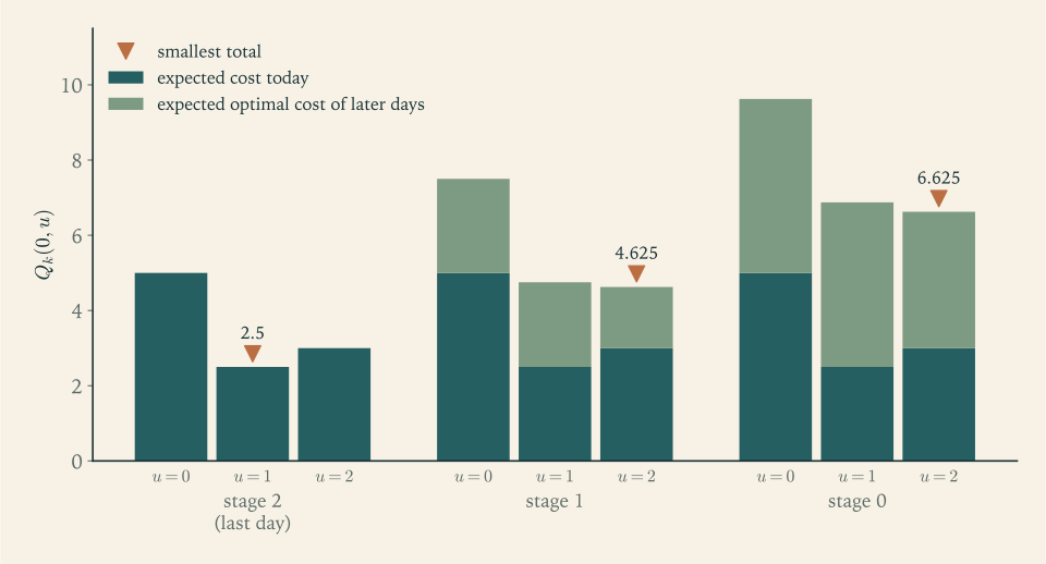
The lower segments are identical in the three groups: they are \(\bar g(0,u)\) . On the last day there is no upper segment and one unit wins. With days remaining, a unit left on the shelf tonight is a unit that need not be bought tomorrow, so the expected future cost falls from \(\tfrac94\) to \(\tfrac{13}{8}\) when the order rises from one to two, a saving of \(\tfrac58\) that outweighs the extra \(\tfrac12\) paid today. On the last day leftover stock is worth nothing, and the saving vanishes. The dependence of the policy on the time remaining is called an end-of-horizon effect.
2.4 Why the short-sighted rule fails
Example 2.2: The price of myopia
A myopic policy chooses at each stage the control that minimizes the expected cost of that stage alone. In the shop this is “order up to one unit” every day, since \(\bar g(0,1)=\tfrac52\) and \(\bar g(1,0)=\tfrac32\) are the smallest entries for their states.
Evaluate it by Lemma 2.1. At stage \(2\) the myopic rule coincides with \(\mu_2^\star\) , so its cost-to-go there is \(\big(\tfrac52,\tfrac32,1\big)\) . At stage \(1\) , from state \(0\) , it orders one unit and pays \(Q_1(0,1)=\tfrac{19}{4}\) ; from state \(1\) it pays \(Q_1(1,0)=\tfrac{15}{4}\) ; from state \(2\) , \(\tfrac{21}{8}\) . At stage \(0\) from an empty shelf,
The optimal cost is \(\tfrac{53}{8}=6.625\) . Myopia costs \(\tfrac38\) over three days, about \(5.7\) percent.
Common mistake. Arguing that a sum is minimized by minimizing each of its terms. That is true when the terms can be chosen independently. Here they cannot: the control chosen at stage \(k\) fixes the distribution of \(x_{k+1}\) , and with it the set of costs that are achievable at stage \(k+1\) . The myopic rule minimizes the first term of \(Q_k(x,u)\) and ignores the second. The repair is mechanical: never compare controls by \(\bar g_k(x,u)\) alone unless \(J_{k+1}\) is constant, as it is at the last stage.
A second error is subtler, because it produces a recursion that looks right. The Bellman recursion takes the minimum of an expectation: the control is chosen first and the disturbance is averaged afterwards. Writing the expectation of a minimum instead,
describes a decision maker who sees \(w_k\) before choosing \(u\) . At the last stage of the shop, from an empty shelf, that decision maker orders exactly the demand and pays \(\tfrac14\cdot 0+\tfrac12\cdot 1+\tfrac14\cdot 2=1\) , against the true \(J_2(0)=\tfrac52\) . The number \(1\) is a correct answer to a different problem. The gap of \(\tfrac32\) is what knowing the demand in advance would be worth, a quantity that Chapter 6 studies under the name of the value of information.
2.5 The principle of optimality and its fine print
Bellman stated the idea behind the recursion as a principle: whatever the first decision and the state it leads to, the remaining decisions of an optimal policy must be optimal for the problem that starts from that state. The policy \(\pi^\star\) of Theorem 2.2 has this property by construction, at every state. For an arbitrary policy that is optimal from one particular initial state the principle needs a qualification.
Proposition 2.3 (principle of optimality). Let \(\pi\) be a policy with \(J_0^{\pi}(x_0)=J_0(x_0)\) for a particular initial state \(x_0\) . If a state \(x\) is reached at stage \(k\) with positive probability when \(\pi\) is used from \(x_0\) , then \(J_k^{\pi}(x)=J_k(x)\) : the tail of \(\pi\) is optimal for the tail subproblem at \((k,x)\) .
Proof. Let \(\tilde\pi\) use the rules \(\mu_0,\dots,\mu_{k-1}\) of \(\pi\) for the first \(k\) stages and the rules \(\mu_k^\star,\dots,\mu_{N-1}^\star\) of Theorem 2.2 afterwards. The two policies generate the same distribution of \(x_k\) and the same expected cost \(c\) over stages \(0\) to \(k-1\) , so
Every term of the first sum is at least the matching term of the second, by Theorem 2.2. If \(J_k^{\pi}(x)\) exceeded \(J_k(x)\) at some \(x\) with \(P(x_k=x)\) positive, then \(J_0^{\tilde\pi}(x_0)\) would be strictly less than \(J_0^{\pi}(x_0)=J_0(x_0)\) , contradicting the theorem.
Example 2.3: An optimal policy that is wrong where it never goes
Example 1.5 found two policies with cost \(\tfrac{53}{8}\) from an empty shelf. Both order two units at \((k,x)=(0,0)\) and agree with the table of Example 2.1 on days \(1\) and \(2\) . They differ at stage \(0\) in state \(1\) : one orders a unit, as the table says, and the other orders nothing.
The Q-factors there are \(Q_0(1,1)=\tfrac{45}{8}\) and \(Q_0(1,0)=\tfrac{47}{8}\) , so the second policy is not optimal for the problem that starts with one unit on the shelf: it loses \(\tfrac14\) . Starting from an empty shelf, however, the state at stage \(0\) is \(0\) and never \(1\) , so the defect is never exercised. This policy satisfies the hypothesis of Proposition 2.3 for \(x_0=0\) and is not an optimal policy in the sense of Definition 1.2, which demands optimality from every initial state.
The distinction matters when a computed policy is used on a real system. A policy obtained by backward induction is correct at every state, including states that a disturbance outside the model might produce. A policy obtained by searching for the best behaviour from one starting point carries no such guarantee.
2.6 Problems with structure, and problems outside the recursion
The recursion is a statement about functions \(J_k\) , and nothing requires those functions to be stored as tables. When the state is a continuous quantity a table is impossible, but sometimes the functions have a formula that the recursion preserves from stage to stage. Finding such a formula is the best possible outcome, because it removes the dependence on the number of states altogether.
Example 2.4: Betting a fraction of one’s wealth
A gambler with wealth \(x_k\) bets a fraction \(u_k\in[0,1)\) of it at even odds on an event that occurs with probability \(p\) , with \(\tfrac12\le p\) and \(p\) less than \(1\) . Wealth becomes \(x_k(1+u_k)\) after a win and \(x_k(1-u_k)\) after a loss. The gambler wants to maximize \(E[\log x_N]\) after \(N\) independent bets. This is a reward problem, so the recursion has a maximum where Theorem 2.2 has a minimum, and the state set is the positive half-line. The induction in the proof of Theorem 2.2 used finiteness only to be sure that the expectations and the minima exist; here they will exist by direct computation.
Start from \(J_N(x)=\log x\) and guess that \(J_k(x)=\log x+(N-k)\,C\) for a constant \(C\) . If this holds at stage \(k+1\) , then
with \(h(u)=p\log(1+u)+(1-p)\log(1-u)\) . The function \(h\) is concave, and \(h'(u)=\dfrac{p}{1+u}-\dfrac{1-p}{1-u}\) vanishes at
So the guess is confirmed, with this \(C\) , and the optimal policy bets the fraction \(2p-1\) of current wealth at every stage, whatever the wealth and however many bets remain.
For \(p=0.6\) the optimal fraction is \(u^\star=0.2\) and \(C\approx 0.0201\) , so ten bets raise the expected logarithm of wealth by \(0.2014\) . Betting twice the optimal fraction is not twice as good: \(h(0.4)\approx-0.0024\) , a negative growth rate from a favourable game.
Here the optimal policy is myopic. That is a property of the logarithm, which turns the product of wealth factors into a sum of independent terms, and it should be read as a warning about generalizing from Example 2.2 in either direction: whether looking ahead matters is decided by the recursion, not by intuition.
The recursion also has limits. Its proof needed the total cost to be assembled from the stage cost and the remainder in a way that is monotone in the remainder. Sums are, and so are maxima: replacing the expectation in Theorem 2.2 by a maximum over \(w_k\) gives a valid recursion for the worst-case cost, with the same proof. Products are monotone only when the factors are nonnegative.
Example 2.5: A product of signed rewards
Two decisions are made in sequence. The first picks a factor \(r_0\in\{-2,\,1\}\) , the second a factor \(r_1\in\{-3,\,1\}\) , and the objective is to maximize the product \(r_0r_1\) . Imitating the recursion, one would solve the tail problem first, \(\max r_1=1\) , and then choose \(r_0\) to maximize \(r_0\cdot 1\) , obtaining \(r_0=1\) and a value of \(1\) .
The four products are \(6\) , \(-2\) , \(-3\) , and \(1\) . The true maximum is \(6\) , attained by \(r_0=-2\) and \(r_1=-3\) , and its tail \(r_1=-3\) is the worst solution of the tail problem. The principle of optimality is false here. The failing step is the first inequality in the proof of Theorem 2.2: when \(r_0\) is negative, a larger remainder gives a smaller total.
The remedy is the remedy of Chapter 1: find a description of the tail that suffices. Here it is enough to carry both the largest and the smallest achievable tail product, \(1\) and \(-3\) , and to compute \(\max\{r_0\cdot 1,\ r_0\cdot(-3)\}\) for each \(r_0\) , which gives \(\max\{-2,6\}=6\) for \(r_0=-2\) and \(\max\{1,-3\}=1\) for \(r_0=1\) .
Two questions lead on from here. The recursion costs one bracket per state, control, and stage; what if there are no disturbances, so that each bracket is a single number? Then the problem is a shortest-path problem, and Chapter 3 exploits that. And what happens to \(J_k\) as the number of remaining stages grows without bound? In the shop, the policy at stages \(0\) and \(1\) was already the same. Chapter 4 shows that with discounting the recursion converges, and to what.
Exercises
-
State the dynamic programming algorithm of Theorem 2.2 from memory, and explain in words what each of \(J_k(x)\) , \(Q_k(x,u)\) , and \(\mu_k^\star(x)\) represents, including which decisions are assumed to be made optimally in each.
Hint
Write the terminal condition first, then the recursion with the minimum outside the expectation. \(J_k(x)\) assumes optimal decisions at stages \(k,k+1,\dots,N-1\) . \(Q_k(x,u)\) assumes the given control \(u\) at stage \(k\) and optimal decisions from stage \(k+1\) on. \(\mu_k^\star(x)\) is a control whose Q-factor is smallest.
-
In the shop of Example 1.1 change the shortage cost from \(5\) to \(3\) per unit. Recompute the expected one-day costs, find \(J_2\) and \(\mu_2^\star\) , and decide by comparing \(Q_1(0,1)\) with \(Q_1(0,2)\) whether an order of two units from an empty shelf is still preferred at stage \(1\) .
Answer
The expected one-day costs become \(\bar g(0,0)=3\) , \(\bar g(0,1)=2\) , \(\bar g(0,2)=3\) , \(\bar g(1,0)=1\) , \(\bar g(1,1)=2\) , \(\bar g(2,0)=1\) . Hence \(J_2=(2,1,1)\) and \(\mu_2^\star=(1,0,0)\) . At stage \(1\) , \(Q_1(0,1)=2+\tfrac14\cdot1+\tfrac34\cdot 2=\tfrac{15}{4}\) and \(Q_1(0,2)=3+\tfrac14\cdot1+\tfrac12\cdot1+\tfrac14\cdot2=\tfrac{17}{4}\) , so one unit is now preferred. With a cheaper shortage the second unit no longer pays for itself.
-
Three units of an indivisible resource are to be divided among three activities. Allocating \(u\) units to activity \(1\) returns \(0,5,8,9\) for \(u=0,1,2,3\) ; activity \(2\) returns \(0,4,9,11\) ; activity \(3\) returns \(0,6,7,12\) . Treat the activities as stages and the units still unallocated as the state, and find the largest total return and every allocation that attains it by a backward recursion.
Solution
Let \(V_k(x)\) be the largest return obtainable from activities \(k,\dots,3\) with \(x\) units still unallocated, and write \(r_k(u)\) for the return of activity \(k\) . The recursion is \(V_k(x)=\max_{0\le u\le x}\big[r_k(u)+V_{k+1}(x-u)\big]\) with \(V_4\equiv 0\) ; there is no disturbance, so there is no expectation.
For the last activity the best use of \(x\) units is the best of \(r_3(0),\dots,r_3(x)\) , giving \(V_3=(0,6,7,12)\) for \(x=0,1,2,3\) .
For activity \(2\) : \(V_2(1)=\max\{0+6,\ 4+0\}=6\) ; \(V_2(2)=\max\{0+7,\ 4+6,\ 9+0\}=10\) ; \(V_2(3)=\max\{0+12,\ 4+7,\ 9+6,\ 11+0\}=15\) . So \(V_2=(0,6,10,15)\) .
For activity \(1\) with all three units: \(V_1(3)=\max\{0+15,\ 5+10,\ 8+6,\ 9+0\}=15\) . The maximum is attained by \(u=0\) and by \(u=1\) . Tracing forward: \(u=0\) leaves \(3\) units, where activity \(2\) takes \(2\) and activity \(3\) takes \(1\) ; \(u=1\) leaves \(2\) units, where activity \(2\) takes \(1\) and activity \(3\) takes \(1\) . The largest total return is \(15\) , attained by the allocations \((0,2,1)\) and \((1,1,1)\) .
-
In the shop of Example 2.1 suppose each unit left at the end of day \(2\) can be returned for a refund of \(1\) , so that \(g_3(x)=-x\) . Recompute the table and explain why the end-of-horizon effect disappears.
Solution
With \(g_3(x)=-x\) the stage-\(2\) Q-factors are the one-day costs minus the expected leftover stock, which is the expected holding quantity. From Example 1.1 that quantity is \(0\) , \(\tfrac14\) , \(1\) for a shelf of \(0\) , \(1\) , \(2\) after ordering. So \(Q_2(0,0)=5\) , \(Q_2(0,1)=\tfrac52-\tfrac14=\tfrac94\) , \(Q_2(0,2)=3-1=2\) ; \(Q_2(1,0)=\tfrac32-\tfrac14=\tfrac54\) , \(Q_2(1,1)=2-1=1\) ; \(Q_2(2,0)=1-1=0\) . Hence \(J_2=(2,1,0)\) with \(\mu_2^\star=(2,1,0)\) : fill the shelf even on the last day.
Now \(J_2(x)=2-x\) , so \(J_2\) at the next state equals \(2\) minus the leftover stock, and the stage-\(1\) Q-factors are \(Q_2(x,u)+2\) . The same holds at stage \(0\) . Therefore \(J_1=(4,3,2)\) , \(J_0=(6,5,4)\) , and the policy is “order up to two” at every stage.
The effect disappears because the refund equals the purchase price. A unit left at the end is no longer wasted; it returns exactly what it cost, so the only penalty for over-ordering is the holding cost, which the last day shares with every other day. The terminal cost has made the last day look like a day with a future.
-
Let two models differ only in their terminal costs, with \(g_N(x)\le g_N'(x)\) for every \(x\) . Prove that \(J_k(x)\le J_k'(x)\) for every stage and state.
Solution
Induct backward. At \(k=N\) , \(J_N=g_N\le g_N'=J_N'\) . Suppose \(J_{k+1}\le J_{k+1}'\) pointwise. For each \(x\) and each \(u\in U_k(x)\) ,
\[ E\big[g_k(x,u,w_k)+J_{k+1}(f_k(x,u,w_k))\big]\le E\big[g_k(x,u,w_k)+J_{k+1}'(f_k(x,u,w_k))\big], \]because the expectation is a sum with nonnegative weights and each term on the left is at most the matching term on the right. Taking the minimum over \(u\) on both sides preserves the inequality: if \(a(u)\le b(u)\) for all \(u\) then \(\min_u a(u)\le a(u^{b})\le b(u^{b})=\min_u b(u)\) , where \(u^{b}\) minimizes \(b\) . Hence \(J_k(x)\le J_k'(x)\) . This monotonicity of the Bellman recursion in its terminal function is the property that drives the proof of Theorem 2.2, and it returns in Chapter 4 as the monotonicity of the operator \(T\) .
-
Prove that adding a constant \(c\) to the terminal cost adds \(c\) to every \(J_k(x)\) and leaves the minimizing controls unchanged, and that multiplying every stage cost and the terminal cost by a constant \(\beta\) greater than \(0\) multiplies every \(J_k(x)\) by \(\beta\) .
Hint
Both parts are backward inductions. For the constant: if \(J_{k+1}'=J_{k+1}+c\) , then every bracket in the recursion increases by exactly \(c\) , because \(c\) passes through the expectation, and a common shift does not change which control is smallest. For the scaling: a positive factor passes through the expectation and through the minimum. Ask yourself where the argument breaks if \(\beta\) is negative.
-
In the setting of Example 2.4 let the gambler maximize \(E[\sqrt{x_N}]\) instead. Show by induction that \(J_k(x)=A^{N-k}\sqrt{x}\) , find the optimal fraction and the constant \(A\) in terms of \(p\) , and evaluate both for \(p=0.6\) .
Solution
Guess \(J_k(x)=A^{N-k}\sqrt x\) , which holds at \(k=N\) . If it holds at \(k+1\) , then
\[ J_k(x)=\max_{0\le u<1}A^{N-k-1}\Big[p\sqrt{x(1+u)}+(1-p)\sqrt{x(1-u)}\Big]=A^{N-k-1}\sqrt x\ \max_{0\le u<1}a(u), \]with \(a(u)=p\sqrt{1+u}+(1-p)\sqrt{1-u}\) . Write \(q=1-p\) . The function \(a\) is concave and \(a'(u)=\dfrac{p}{2\sqrt{1+u}}-\dfrac{q}{2\sqrt{1-u}}\) vanishes when \(p^{2}(1-u)=q^{2}(1+u)\) , that is, at
\[ u^\star=\frac{p^{2}-q^{2}}{p^{2}+q^{2}}=\frac{2p-1}{p^{2}+q^{2}} . \]At that point \(1+u^\star=\dfrac{2p^{2}}{p^{2}+q^{2}}\) and \(1-u^\star=\dfrac{2q^{2}}{p^{2}+q^{2}}\) , so
\[ A=a(u^\star)=\frac{\sqrt2\,(p^{2}+q^{2})}{\sqrt{p^{2}+q^{2}}}=\sqrt{2(p^{2}+q^{2})}. \]The induction closes with this \(A\) . For \(p=0.6\) : \(p^{2}+q^{2}=0.52\) , so \(u^\star=\tfrac{5}{13}\approx 0.385\) and \(A=\sqrt{1.04}\approx 1.0198\) .
The square-root gambler bets nearly twice the fraction of the logarithmic gambler, \(0.385\) against \(0.2\) . The square root is less concave than the logarithm, so it penalizes losses less, and the policy is correspondingly bolder. As in Example 2.4 the optimal fraction does not depend on the stage or on wealth.
-
A student claims: “At each stage I choose the order with the smallest expected cost for that day. Each term of the total is then as small as it can be, so the total is as small as it can be.” Identify the false step, and give the two numbers from the shop that refute the conclusion.
Solution
The false step is “each term is as small as it can be”. The smallest value available for the cost of day \(k+1\) depends on the state in which day \(k+1\) begins, and that state is determined, in distribution, by the order chosen on day \(k\) . Minimizing the cost of day \(k\) over the order can therefore raise the cost of day \(k+1\) : the terms are coupled through the state and cannot be minimized separately.
In the shop the rule described is “order up to one unit” on every day. By Example 2.2 its three-day cost from an empty shelf is \(7\) , while the optimal cost is \(J_0(0)=\tfrac{53}{8}=6.625\) . The rule’s first-day cost, \(\tfrac52\) , is indeed smaller than the \(3\) paid by the optimal policy on the first day; the optimal policy recovers more than the difference on the later days, because it starts them with more stock.
-
A student implementing the recursion for the shop computes, at the last stage from an empty shelf, the average over demand of the smallest cost achievable for that demand, and reports \(1\) . Explain what decision problem this number solves, why it is not \(J_2(0)\) , and why it is smaller.
Answer
It solves the problem in which the manager sees the day’s demand before ordering: with demand \(w\) the best order is \(w\) at cost \(w\) , and the average is \(\tfrac14\cdot0+\tfrac12\cdot1+\tfrac14\cdot2=1\) . It is not \(J_2(0)=\tfrac52\) because the model’s order of events puts the control before the disturbance. It is smaller because a minimum taken separately for each \(w\) is at most the value, at that \(w\) , of any single control, so the average of the minima is at most the minimum of the averages.
-
Using the Q-factors \(Q_0(1,0)\) and \(Q_0(1,1)\) of the shop, exhibit a policy that attains \(J_0(0)\) from an empty shelf but is not optimal in the sense of Definition 1.2, compute the cost it incurs from \(x_0=1\) , and explain why this does not contradict Proposition 2.3.
Solution
Let \(\pi\) agree with the table of Example 2.1 everywhere except that \(\mu_0(1)=0\) . From \(x_0=0\) the state at stage \(0\) is \(0\) , the rule \(\mu_0(1)\) is never consulted, and \(\pi\) behaves exactly like \(\pi^\star\) ; so \(J_0^{\pi}(0)=\tfrac{53}{8}=J_0(0)\) .
From \(x_0=1\) the policy orders nothing at stage \(0\) and then follows the optimal rules, so its cost is the Q-factor \(Q_0(1,0)=\tfrac{47}{8}\) . The optimal cost is \(J_0(1)=Q_0(1,1)=\tfrac{45}{8}\) . The policy loses \(\tfrac14\) from that starting state and so is not optimal in the sense of Definition 1.2.
There is no contradiction with Proposition 2.3. Its hypothesis is optimality from a particular \(x_0\) , here \(x_0=0\) , and its conclusion concerns only the pairs \((k,x)\) reached with positive probability from that \(x_0\) . At stage \(0\) the only such state is \(0\) . At stages \(1\) and \(2\) all three states are reached with positive probability after an order of two units, and there \(\pi\) is optimal, as the proposition requires.
-
Replace the expectation in the shop’s recursion by the maximum over the three demand values, so that the manager guards against the worst case. Compute the worst-case cost-to-go at stage \(2\) and the minimizing orders, and compare the policy with \(\mu_2^\star\) of Example 2.1.
Answer
The worst-case one-day costs are \(\max_w g(0,0,w)=10\) , \(\max_w g(0,1,w)=6\) , \(\max_w g(0,2,w)=4\) ; \(\max_w g(1,0,w)=5\) , \(\max_w g(1,1,w)=3\) ; \(\max_w g(2,0,w)=2\) . The worst-case cost-to-go at stage \(2\) is \((4,3,2)\) and the minimizing orders are \((2,1,0)\) : fill the shelf. The expected-cost policy \(\mu_2^\star=(1,0,0)\) accepts a one-in-four chance of a shortage; the worst-case policy does not.
-
Write the recursion for the shop in transition-probability form, giving \(p_{0j}(2)\) and \(\bar g(0,2)\) explicitly, and use it to recompute \(Q_1(0,2)\) .
Answer
\(p_{02}(2)=\tfrac14\) , \(p_{01}(2)=\tfrac12\) , \(p_{00}(2)=\tfrac14\) , and \(\bar g(0,2)=3\) . Then \(Q_1(0,2)=3+\tfrac14\cdot1+\tfrac12\cdot\tfrac32+\tfrac14\cdot\tfrac52=\tfrac{37}{8}\) , as in Example 2.1.
-
For a model with stage costs \(\alpha^{k}g(x,u,w)\) , where \(\alpha\in(0,1)\) , define \(\tilde J_k(x)=\alpha^{-k}J_k(x)\) . Show that \(\tilde J_k(x)=\min_{u}E[g(x,u,w)+\alpha\,\tilde J_{k+1}(f(x,u,w))]\) , and say why this form is more convenient when the model is otherwise the same at every stage.
Hint
Substitute \(J_k=\alpha^{k}\tilde J_k\) and \(J_{k+1}=\alpha^{k+1}\tilde J_{k+1}\) into the recursion of Theorem 2.2 and divide by \(\alpha^{k}\) , which is positive and so passes through the minimum. The functions \(\tilde J_k\) are costs measured in the money of stage \(k\) . Their recursion uses the same bracket at every stage, which is what makes it possible to let the number of stages grow in Chapter 4.
-
A model has \(n\) states, \(m\) controls in each state, \(d\) disturbance values, and \(N\) stages. Count the additions and multiplications that the recursion of Theorem 2.2 performs, to leading order, and evaluate the count for \(n=1000\) , \(m=20\) , \(d=50\) , \(N=100\) .
Answer
Each Q-factor is a sum of \(d\) products, each product needing one evaluation of \(g_k+J_{k+1}\) : about \(d\) multiplications and \(2d\) additions. There are \(N\,n\,m\) Q-factors, so the count is of order \(N\,n\,m\,d\) . For the given sizes that is \(100\cdot1000\cdot20\cdot50=10^{8}\) brackets’ worth of terms, a fraction of a second of machine time, for a problem with \(20^{100{,}000}\) policies.
-
Return to Example 1.3 with the augmented state “idle” or “running”, a demand of exactly one unit on each day, a making cost of \(1\) , a start-up cost of \(3\) , and a buying price of \(3\) . With the machine idle at the outset, find the optimal cost and the optimal first action for horizons of \(1\) , \(2\) , and \(3\) days by backward induction.
Solution
Let \(J_j(s)\) be the optimal cost with \(j\) days remaining and machine state \(s\) . With no days left the cost is \(0\) . On each day the unit is either bought, at cost \(3\) , after which the machine is idle, or made, at cost \(1\) plus the start-up cost \(3\) if the machine is idle, after which the machine is running.
If the machine is running, making costs \(1\) per day and buying costs \(3\) , so \(J_j(\text{running})=j\) : keep making.
If the machine is idle: with one day left, \(J_1(\text{idle})=\min\{3,\ 4\}=3\) , attained by buying. With two days left, \(J_2(\text{idle})=\min\{3+J_1(\text{idle}),\ 4+J_1(\text{running})\}=\min\{3+3,\ 4+1\}=5\) , attained by making. With three days left, \(J_3(\text{idle})=\min\{3+J_2(\text{idle}),\ 4+J_2(\text{running})\}=\min\{3+5,\ 4+2\}=6\) , attained by making.
So the optimal cost is \(3\) , \(5\) , \(6\) for horizons of \(1\) , \(2\) , \(3\) days, and the optimal first action is to buy when one day remains and to start the machine when two or more remain. The start-up cost is an investment that needs at least two days of use to repay, and only the augmented state lets the recursion see it.
-
A gambler with wealth \(x\in\{0,1,2,3,4\}\) may stake any whole amount \(u\) with \(u\le x\) and \(u\le 4-x\) on an event of probability \(0.4\) at even odds, and wants to maximize the probability of holding \(4\) after at most two bets. Compute the optimal probability from each wealth by backward induction and describe the optimal first stake from wealth \(2\) and from wealth \(3\) .
Solution
Let \(V_j(x)\) be the largest probability of holding \(4\) when \(j\) bets remain. \(V_0(x)=1\) if \(x=4\) and \(0\) otherwise, and \(V_j(x)=\max_u\big[0.4\,V_{j-1}(x+u)+0.6\,V_{j-1}(x-u)\big]\) over the admissible stakes; a stake of \(0\) is admissible.
One bet remaining: from \(2\) the stake \(2\) wins with probability \(\tfrac25\) ; from \(1\) or \(3\) no admissible stake reaches \(4\) except the stake \(1\) from \(3\) , which gives \(\tfrac25\) . So \(V_1=\big(0,0,\tfrac25,\tfrac25,1\big)\) .
Two bets remaining: from \(1\) , stake \(1\) to reach \(2\) with probability \(\tfrac25\) and then win again: \(V_2(1)=\tfrac25\cdot\tfrac25=\tfrac{4}{25}\) . From \(2\) : stake \(2\) gives \(\tfrac25\) ; stake \(1\) gives \(\tfrac25V_1(3)+\tfrac35V_1(1)=\tfrac{4}{25}\) ; stake \(0\) gives \(V_1(2)=\tfrac25\) . From \(3\) : stake \(1\) gives \(\tfrac25\cdot1+\tfrac35V_1(2)=\tfrac25+\tfrac{6}{25}=\tfrac{16}{25}\) ; stake \(0\) gives \(\tfrac25\) . Hence
\[ V_2=\big(0,\tfrac{4}{25},\tfrac25,\tfrac{16}{25},1\big). \]From wealth \(2\) the optimal first stake is the whole \(2\) , or equally a stake of \(0\) followed by the whole \(2\) ; the timid stake of \(1\) is strictly worse. From wealth \(3\) the optimal first stake is \(1\) , exactly the amount needed to reach the goal. In an unfavourable game the best policy makes as few bets as possible.
-
Suppose the admissible control sets do not depend on the state, so that every open-loop plan is admissible from every state. Prove that the optimal cost \(J_0(x_0)\) is no larger than the expected cost of the best open-loop plan.
Solution
Let \((u_0,\dots,u_{N-1})\) be the best open-loop plan. Because the admissible sets do not depend on the state, the constant functions \(\mu_k(x)=u_k\) form a policy \(\pi\) in the sense of Definition 1.2: each \(\mu_k(x)\) is admissible at every \(x\) . Under this policy the control applied at stage \(k\) is \(u_k\) on every disturbance path, exactly as under the plan, so the two generate the same states and the same costs path by path, and \(J_0^{\pi}(x_0)\) equals the expected cost of the plan. By Theorem 2.2, \(J_0(x_0)\le J_0^{\pi}(x_0)\) . Hence the optimal cost is at most the cost of the best plan. The hypothesis on the admissible sets is needed only to make the plan a legitimate policy; in the shop, where the capacity constraint depends on the stock, the same conclusion holds for the plans that are feasible on every path, as in Example 1.2.
-
In Example 2.4 suppose \(p\) is at most \(\tfrac12\) . Show that \(h\) is maximized over \(0\le u\) at \(u=0\) , find \(J_k\) , and interpret the result.
Answer
For \(p\le\tfrac12\) , \(h'(u)=\dfrac{p}{1+u}-\dfrac{1-p}{1-u}\) is at most \(2p-1\le 0\) at \(u=0\) and decreases as \(u\) grows, so \(h\) is maximized at \(u=0\) with \(h(0)=0\) . Then \(C=0\) and \(J_k(x)=\log x\) : in a fair or unfavourable game the logarithmic gambler does not bet at all.