Remove the disturbance from the model of Chapter 1 and three things happen at once. The expectation in the Bellman recursion disappears, so each Q-factor is a single sum. By Proposition 1.3 a policy has no advantage over a plan from a fixed starting state, so the problem is to find one good sequence of controls. And a sequence of controls is a path: through a graph whose nodes are pairs of stage and state and whose arcs are the admissible transitions. A deterministic sequential decision problem is a shortest-path problem.
That observation cuts both ways. It lets this chapter borrow the language of graphs, and it shows that the recursion of Chapter 2 is, among other things, a shortest-path algorithm. The chapter then follows two directions in which the deterministic case goes further than the stochastic one. The first is feasibility: when some states are forbidden or a target must be reached, the same backward sweep that computes costs also computes the set of states from which the target can be reached at all. The second is the continuous state. For linear dynamics and quadratic costs the cost-to-go functions are quadratic forms, the table is replaced by a matrix recursion, and the optimal policy is a linear feedback. This is the linear-quadratic regulator, the most used result in control.
3.1 Sequential decisions as paths
With no disturbance the recursion of Theorem 2.2 reads
Build a graph with one node for each pair \((k,x)\) , an arc from \((k,x)\) to \((k+1,f_k(x,u))\) of length \(g_k(x,u)\) for each admissible \(u\) , and an arc of length \(g_N(x)\) from each \((N,x)\) to an artificial terminal node \(t\) . A sequence of controls from \(x_0\) is a path from \((0,x_0)\) to \(t\) , its cost is the length of the path, and \(J_k(x)\) is the length of a shortest path from \((k,x)\) to \(t\) . The recursion says: the shortest distance from a node is the smallest, over outgoing arcs, of the arc length plus the shortest distance from the arc’s head.
Shortest-path problems on general graphs, with the algorithms of Dijkstra and others, are developed in Discrete Optimization (math.discrete-optimization.shortest-path-flow). What this chapter adds is the reading of the recursion as one such algorithm, and two extensions that the staged structure makes easy.
Example 3.1: A staged network, backward and forward
A route runs from \(s\) to \(t\) through three intermediate stages with nodes \(a_1,a_2\) , then \(b_1,b_2,b_3\) , then \(c_1,c_2\) . The arc lengths are
| From | To and length |
|---|---|
| \(s\) | \(a_1\) : \(2\) , \(a_2\) : \(3\) |
| \(a_1\) | \(b_1\) : \(7\) , \(b_2\) : \(4\) , \(b_3\) : \(6\) |
| \(a_2\) | \(b_1\) : \(3\) , \(b_2\) : \(4\) , \(b_3\) : \(4\) |
| \(b_1\) | \(c_1\) : \(1\) , \(c_2\) : \(4\) |
| \(b_2\) | \(c_1\) : \(6\) , \(c_2\) : \(3\) |
| \(b_3\) | \(c_1\) : \(3\) , \(c_2\) : \(3\) |
| \(c_1\) , \(c_2\) | \(t\) : \(4\) and \(t\) : \(3\) |
Backward. \(J(c_1)=4\) and \(J(c_2)=3\) . Then \(J(b_1)=\min\{1+4,\,4+3\}=5\) , \(J(b_2)=\min\{6+4,\,3+3\}=6\) , \(J(b_3)=\min\{3+4,\,3+3\}=6\) . Then \(J(a_1)=\min\{7+5,\,4+6,\,6+6\}=10\) and \(J(a_2)=\min\{3+5,\,4+6,\,4+6\}=8\) . Finally \(J(s)=\min\{2+10,\,3+8\}=11\) . Following the minimizing arcs forward from \(s\) gives the path \(s\to a_2\to b_1\to c_1\to t\) with length \(3+3+1+4=11\) .
A traveller who takes the shortest arc at each node goes \(s\to a_1\to b_2\to c_2\to t\) , with length \(2+4+3+3=12\) . The first arc of that route is the shorter of the two leaving \(s\) , and it leads to the node with the larger cost-to-go.
Forward. Let \(D(i)\) be the shortest distance from \(s\) to node \(i\) . Then \(D(a_1)=2\) , \(D(a_2)=3\) ; \(D(b_1)=\min\{2+7,\,3+3\}=6\) , \(D(b_2)=\min\{2+4,\,3+4\}=6\) , \(D(b_3)=\min\{2+6,\,3+4\}=7\) ; \(D(c_1)=\min\{6+1,\,6+6,\,7+3\}=7\) , \(D(c_2)=\min\{6+4,\,6+3,\,7+3\}=9\) ; and \(D(t)=\min\{7+4,\,9+3\}=11\) . The two sweeps agree, as they must.
There are \(2\cdot3\cdot2=12\) routes. The backward sweep examined each of the \(16\) arcs once.
The forward sweep of the example is available because a path from \(s\) to \(t\) is also a path from \(t\) to \(s\) in the graph with every arc reversed, and the backward recursion in the reversed graph is the forward recursion in the original.
Proposition 3.1 (forward recursion). In a deterministic finite problem with a given initial state \(x_0\) , define \(D_0(x_0)=0\) and, for \(k=0,\dots,N-1\) and each \(y\in S_{k+1}\) ,
with the minimum over an empty set equal to \(+\infty\) . Then \(D_k(x)\) is the smallest cost of reaching \(x\) at stage \(k\) from \(x_0\) , and \(J_0(x_0)=\min_{x\in S_N}\big[D_N(x)+g_N(x)\big]\) .
Proof. By induction on \(k\) . A cheapest way to be at \(y\) at stage \(k+1\) arrives from some state \(x\) at stage \(k\) by some control \(u\) , and the part of it before stage \(k\) must be a cheapest way of reaching \(x\) , since otherwise replacing that part would give a cheaper way of reaching \(y\) . So its cost is \(D_k(x)+g_k(x,u)\) for the best such pair. The final formula splits each complete trajectory into its cost up to stage \(N\) and its terminal cost.
The forward form is the natural one when the initial state is known and the terminal state is free, or when data for later stages arrive only as the computation proceeds. It has no stochastic counterpart. With disturbances, “the cost of reaching \(x\) ” is not a property of \(x\) that can be minimized, because the controller does not choose where the system goes; only the backward recursion, which conditions on where the system is, survives.
3.2 Graphs without stages
Many path problems have no natural stage: the route may use any number of arcs and may revisit nodes. Let the nodes be \(1,\dots,n\) with destination \(t=n\) , and let \(a_{ij}\) be the length of the arc from \(i\) to \(j\) , with \(a_{ij}=+\infty\) when there is no arc. The recursion can still be run, with the iteration counter playing the part of the stage.
Theorem 3.2 (shortest paths by successive approximation). Assume every cycle of the graph has nonnegative length. Set \(J_0(t)=0\) and \(J_0(i)=+\infty\) for \(i\ne t\) , and for \(k=0,1,2,\dots\) let
Then \(J_k(i)\) is the length of a shortest path from \(i\) to \(t\) among paths with at most \(k\) arcs, and \(+\infty\) if there is none. Moreover \(J_{n-1}(i)\) is the length \(J^\star(i)\) of a shortest path with any number of arcs, the iteration is stationary from \(k=n-1\) on, and \(J^\star\) satisfies Bellman’s equation \(J^\star(i)=\min_j\big[a_{ij}+J^\star(j)\big]\) for \(i\ne t\) , with \(J^\star(t)=0\) .
Proof. The first claim is Theorem 2.2 applied to the \(k\) -stage problem in which the state is a node, a control is the choice of the next node, node \(t\) may be kept at zero cost, and the terminal cost is \(0\) at \(t\) and \(+\infty\) elsewhere: a finite cost means that \(t\) has been reached within \(k\) arcs. For the second, take any path from \(i\) to \(t\) that repeats a node. The portion between the two visits is a cycle of nonnegative length, and deleting it gives a path that is no longer. Repeating this produces a path with no repeated node, hence with at most \(n-1\) arcs. So a shortest path with at most \(n-1\) arcs is shortest overall, \(J_{n-1}=J^\star\) , and allowing more arcs changes nothing. Bellman’s equation is the statement \(J_n=J_{n-1}\) .
This is the Bellman–Ford method, seen as dynamic programming. The hypothesis is needed: around a cycle of negative length a path can lower its cost without limit, the iterates decrease for ever, and no shortest path exists.
Example 3.2: Four iterations on a graph with cycles
Take nodes \(1,2,3,4\) and destination \(t=5\) , with arcs \(1\to2\) of length \(1\) , \(1\to3\) of length \(5\) , \(2\to1\) of length \(1\) , \(2\to3\) of length \(1\) , \(2\to4\) of length \(6\) , \(3\to4\) of length \(1\) , \(3\to t\) of length \(7\) , \(4\to2\) of length \(2\) , and \(4\to t\) of length \(1\) . The graph contains the cycles \(1\to2\to1\) and \(2\to3\to4\to2\) , both of positive length.
| \(k\) | \(J_k(1)\) | \(J_k(2)\) | \(J_k(3)\) | \(J_k(4)\) |
|---|---|---|---|---|
| \(0\) | \(\infty\) | \(\infty\) | \(\infty\) | \(\infty\) |
| \(1\) | \(\infty\) | \(\infty\) | \(7\) | \(1\) |
| \(2\) | \(12\) | \(7\) | \(2\) | \(1\) |
| \(3\) | \(7\) | \(3\) | \(2\) | \(1\) |
| \(4\) | \(4\) | \(3\) | \(2\) | \(1\) |
For instance \(J_2(2)=\min\{1+J_1(1),\,1+J_1(3),\,6+J_1(4)\}=\min\{\infty,8,7\}=7\) , the two-arc path through node \(4\) , and \(J_3(2)=\min\{1+12,\,1+2,\,6+1\}=3\) , the three-arc path \(2\to3\to4\to t\) . A fifth iteration reproduces the fourth row. The shortest path from node \(1\) is \(1\to2\to3\to4\to t\) , with \(4=n-1\) arcs and length \(4\) : the bound in the theorem is attained.
3.3 Targets, obstacles, and the states that can reach the goal
Suppose the system must be in a target set \(A\subseteq S_N\) at the final stage, and must avoid certain states on the way. Both requirements fit the recursion through one convention: a forbidden outcome has cost \(+\infty\) . Set \(g_N(x)=+\infty\) for \(x\notin A\) , remove from \(U_k(x)\) any control that leads to a forbidden state, and let the minimum over an empty set be \(+\infty\) . Arithmetic with \(+\infty\) follows the rules \(c+\infty=\infty\) for every finite \(c\) and \(\min\{c,\infty\}=c\) ; no subtraction of infinities ever occurs, because costs are only added and compared.
Definition 3.3 (backward reachable set). For a deterministic problem with target set \(A\) , let \(R_N=A\) and, for \(k=N-1,\dots,0\) ,
\(R_k\) is the set of states at stage \(k\) from which some admissible control sequence brings the system into \(A\) at stage \(N\) .
Proposition 3.4 (feasibility is finiteness of the cost-to-go). Let all stage costs be finite and let \(g_N\) be finite on \(A\) and \(+\infty\) off it. Then for every \(k\) and \(x\in S_k\) , \(J_k(x)\) is finite if and only if \(x\in R_k\) .
Proof. By backward induction. At \(k=N\) the claim is the definition of \(g_N\) . If it holds at \(k+1\) , then \(g_k(x,u)+J_{k+1}(f_k(x,u))\) is finite exactly for those \(u\in U_k(x)\) with \(f_k(x,u)\in R_{k+1}\) , and a minimum of finitely many extended numbers is finite exactly when one of them is. That is the condition defining \(R_k\) .
So a single backward sweep answers two questions: from where is the task possible, and what does it cost from there. The reachable sets are also worth computing on their own, with every cost set to zero, when only safety or feasibility is at stake.
Example 3.3: A robot on a grid
A robot moves on a grid of \(5\) rows and \(7\) columns; cell \((r,c)\) is in row \(r\) , counted from the top, and column \(c\) . Ten cells are walls. A move goes one cell north, south, east, or west into a cell that is not a wall. Entering an ordinary cell costs \(1\) , and entering either of the two sand cells \((3,5)\) and \((4,5)\) costs \(3\) . The target is cell \((1,7)\) , and the number of moves is not limited. This is the setting of Theorem 3.2 with a node for each of the \(25\) free cells.
Iterating \(J_{k+1}(x)=\min_{x'}\big[c(x')+J_k(x')\big]\) over the neighbours \(x'\) of \(x\) , where \(c(x')\) is the cost of entering \(x'\) , starting from \(0\) at the target and \(+\infty\) elsewhere, the values stop changing after \(12\) sweeps. The result, with walls marked, is
| Row | Col. 1 | Col. 2 | Col. 3 | Col. 4 | Col. 5 | Col. 6 | Col. 7 |
|---|---|---|---|---|---|---|---|
| \(1\) | \(12\) | \(11\) | \(10\) | wall | \(2\) | \(1\) | \(0\) |
| \(2\) | \(13\) | wall | \(9\) | wall | \(3\) | wall | \(1\) |
| \(3\) | \(14\) | wall | \(8\) | \(7\) | \(4\) | \(3\) | \(2\) |
| \(4\) | wall | wall | \(9\) | wall | \(7\) | wall | \(3\) |
| \(5\) | \(\infty\) | wall | \(8\) | \(7\) | \(6\) | \(5\) | \(4\) |
Cell \((5,1)\) is shut in by walls: its value stays at \(+\infty\) , and by Proposition 3.4 that is a proof that the target cannot be reached from it. The other \(24\) free cells can reach the target.
From cell \((3,3)\) the optimal route goes east through the sand cell \((3,5)\) at cost \(1+3+1+1+1+1=8\) . The route that avoids sand goes down and around through row \(5\) and costs \(10\) . From the neighbouring cell \((4,3)\) the two directions tie at \(9\) .
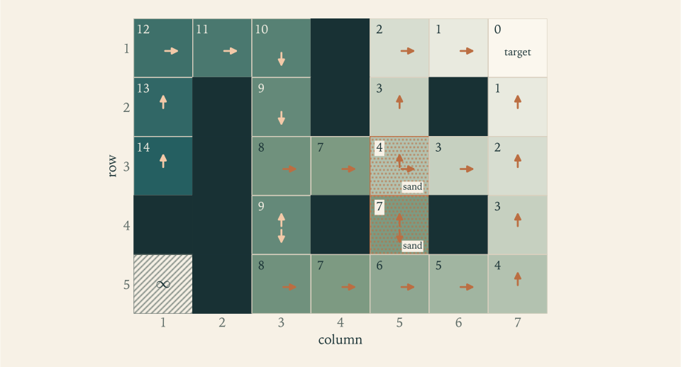
Figure 3.1 makes visible something a list of controls cannot. The arrows are a policy. A robot pushed off its route by an unmodelled bump does not need a new computation; it reads the arrow in the cell where it finds itself. The price is that the whole table had to be computed, although a single trip uses a small part of it.
If the number of moves is limited to \(N\) , the reachable set \(R_0\) of Definition 3.3 is the set of cells with a path of at most \(N\) arcs to the target, provided the robot may wait at the target. Counting from the sweeps of this example, \(1\) , \(3\) , \(5\) , and \(8\) cells can reach the target within \(0\) , \(1\) , \(2\) , and \(3\) moves.
3.4 Linear dynamics and quadratic cost
Now let the state be a vector \(x_k\in\mathbb R^{n}\) and the control an unconstrained vector \(u_k\in\mathbb R^{m}\) , with
The matrices \(Q\) and \(Q_N\) are symmetric positive semidefinite and penalize deviation of the state from the origin; \(R\) is symmetric positive definite and penalizes control effort. The problem is to bring the state near zero without spending too much control: a regulator.
No table can hold \(J_k\) , since the state set is all of \(\mathbb R^{n}\) . The recursion of Theorem 2.2 still makes sense as long as each minimum is attained, and its inductive proof goes through unchanged. What makes the problem tractable is that the recursion preserves a formula.
Theorem 3.5 (discrete-time linear-quadratic regulator). Let \(Q\succeq0\) , \(Q_N\succeq0\) , and \(R\succ0\) . Define symmetric matrices by \(K_N=Q_N\) and the Riccati recursion
Then every \(K_k\) is positive semidefinite, the optimal cost-to-go is \(J_k(x)=x^{\top}K_kx\) , and the unique optimal policy is the linear feedback
Proof. By backward induction. \(J_N(x)=x^{\top}Q_Nx\) with \(K_N=Q_N\succeq0\) . Suppose \(J_{k+1}(x)=x^{\top}K_{k+1}x\) with \(K_{k+1}\succeq0\) , and write \(K=K_{k+1}\) . The quantity to be minimized over \(u\) is
with \(M=R+B^{\top}KB\) . Since \(R\succ0\) and \(B^{\top}KB\succeq0\) , the matrix \(M\) is positive definite, so this is a strictly convex quadratic function of \(u\) . Its gradient \(2Mu+2B^{\top}KAx\) vanishes only at \(u=-M^{-1}B^{\top}KAx=-L_kx\) , and that point is the unique minimizer. Substituting,
The matrix \(K_k\) is symmetric by its formula, and it is positive semidefinite because \(J_k(x)\) , a minimum of nonnegative numbers, is nonnegative for every \(x\) .
The step “the gradient vanishes only at the minimizer” is the first-order characterization of the minimizer of a strictly convex differentiable function from Continuous Optimization (math.continuous-optimization.unconstrained-optimality). Everything else is algebra, and three features of the result are worth more than the algebra. The optimal control is a linear function of the state. The gains \(L_k\)
do not depend on the initial state, so they can be computed once, before the system runs. And the computation is a recursion on \(n\times n\)
matrices, with a cost that grows like \(n^{3}\)
per stage in place of the exponential growth of a table over a grid in \(\mathbb R^{n}\)
. The curse of dimensionality has been avoided by structure.
Example 3.4: The scalar regulator and the Fibonacci numbers
Let \(x_{k+1}=x_k+u_k\) with cost \(x_N^{2}+\sum_{k=0}^{N-1}(x_k^{2}+u_k^{2})\) , so that \(A=B=Q=R=Q_N=1\) . The Riccati recursion becomes
With \(N=4\) , working backward from \(K_4=1\) :
and the gains are \(L_3=\tfrac12\) , \(L_2=\tfrac35\) , \(L_1=\tfrac{8}{13}\) , \(L_0=\tfrac{21}{34}\) . Each \(K_k\) is a ratio of two consecutive Fibonacci numbers.
From \(x_0=1\) the closed-loop state obeys \(x_{k+1}=(1-L_k)x_k\) :
with controls \(u_0=-\tfrac{21}{34}\) , \(u_1=-\tfrac{4}{17}\) , \(u_2=-\tfrac{3}{34}\) , \(u_3=-\tfrac{1}{34}\) . Adding \(x_k^{2}+u_k^{2}\) over the four stages and \(x_4^{2}\) at the end gives \(\tfrac{55}{34}\approx1.6176\) , which is \(K_0x_0^{2}\) as the theorem asserts.
As the number of remaining stages grows, \(K_k\) approaches the positive solution of \(K=1+\dfrac{K}{1+K}\) , that is, of \(K^{2}-K-1=0\) : the golden ratio \(\tfrac12(1+\sqrt5)\approx1.6180\) . Four stages from the end, \(K_0\) already agrees with it to three decimal places.
Common mistake. Running the Riccati recursion in the wrong direction, or pairing a gain with the wrong matrix. The recursion starts at the terminal cost and goes backward, and the gain used at stage \(k\) is built from \(K_{k+1}\) , the cost-to-go of the state the control leads to. Using \(K_k\) in its place prices the next state as if one more stage of cost lay beyond it, and when the terminal cost is modest, as in Example 3.4, the resulting feedback is too strong. A quick check is the last stage: \(L_{N-1}\) must depend on \(Q_N\) and on nothing else from the recursion.
Example 3.5: A double integrator
A cart on a track has position \(x^{(1)}\) and velocity \(x^{(2)}\) ; over one time step the position advances by the velocity and the velocity by the applied force \(u\) :
Only the position is penalized. Starting from \(K_N=Q\) , the first backward step has \(B^{\top}K_NA=(0,0)\) , so \(L_{N-1}=(0,0)\) and
A force applied at the last stage changes only the final velocity, which carries no cost, so it is not worth applying. For the second step, \(R+B^{\top}K_{N-1}B=2\) and \(B^{\top}K_{N-1}A=(1,2)\) , giving \(L_{N-2}=\big(\tfrac12,1\big)\) and
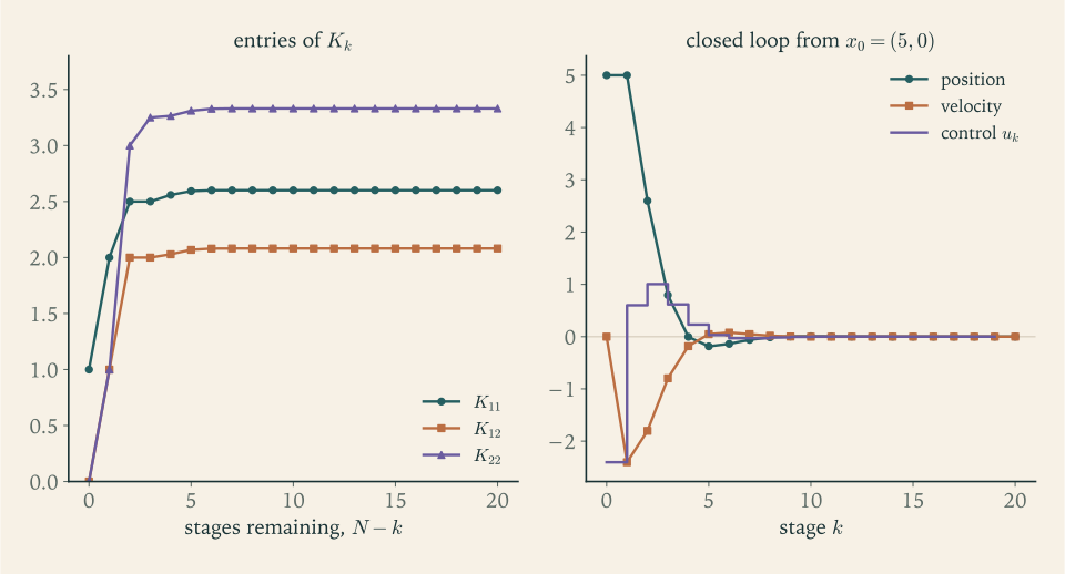
A third step gives \(L_{N-3}=\big(\tfrac12,\tfrac54\big)\) and \(K_{N-3}=\begin{pmatrix}\tfrac52&2\\2&\tfrac{13}{4}\end{pmatrix}\) . Continuing, the matrices settle quickly:
and the closed-loop matrix \(A-BL_\infty\) has the complex pair of eigenvalues \(0.3752\pm0.3002\,i\) , of modulus \(0.4805\) . The state therefore contracts by roughly half at every step.
3.5 Long horizons and the stationary gain
Figure 3.2 and the golden ratio of Example 3.4 show the same thing. Far from the end of the horizon the matrices \(K_k\) no longer change, and their limit satisfies the Riccati recursion with both sides equal, the algebraic Riccati equation
The limit does not always exist, and when it exists the resulting feedback does not always stabilize the system. Two conditions from linear systems theory guarantee both. The pair \((A,B)\) is controllable if the \(n\times nm\) matrix \(\big(B\ \ AB\ \ \cdots\ \ A^{n-1}B\big)\) has rank \(n\) . The rank condition holds exactly when every state can be steered to every other state in \(n\) steps; in particular it implies that every state can be driven to the origin, though that weaker property can hold without it, as the system with \(A=0\) and \(B=0\) shows. Writing \(Q=C^{\top}C\) , the pair \((A,C)\) is observable if the matrix with blocks \(C,CA,\dots,CA^{n-1}\) stacked vertically has rank \(n\) , which means no nonzero trajectory of the uncontrolled system is invisible to the cost.
Theorem 3.6 (stationary regulator). Let \(R\succ0\) and \(Q=C^{\top}C\) , with \((A,B)\) controllable and \((A,C)\) observable. Then for every \(Q_N\succeq0\) the matrices of the Riccati recursion, indexed by the number of stages remaining, converge to a matrix \(K_\infty\) that is the unique positive semidefinite solution of the algebraic Riccati equation. With \(L_\infty=(R+B^{\top}K_\infty B)^{-1}B^{\top}K_\infty A\) , every eigenvalue of \(A-BL_\infty\) has modulus less than \(1\) , and the policy \(\mu(x)=-L_\infty x\) minimizes \(\sum_{k=0}^{\infty}(x_k^{\top}Qx_k+u_k^{\top}Ru_k)\) , with minimum value \(x_0^{\top}K_\infty x_0\) .
The proof needs tools from linear systems theory that this book does not develop, and it is omitted; Exercise 12 proves the scalar case. In Example 3.5 both rank conditions hold, with \(C=(1\ \ 0)\) : the matrices \((B\ \ AB)\) and the stack of \(C\) and \(CA\) are \(\begin{pmatrix}0&1\\1&1\end{pmatrix}\) and \(\begin{pmatrix}1&0\\1&1\end{pmatrix}\) , each of rank \(2\) .
The quadratic cost is forgiving of small errors in the gain. In Example 3.4, using the stationary gain \(L_\infty\approx0.618\) at all four stages, in place of the optimal time-varying gains, raises the cost from \(1.61765\) to \(1.61775\) . The cost is quadratic in the deviation of the gain from its optimum, so a gain that is slightly wrong is very nearly as good; that is one reason the stationary regulator is used so widely even on finite horizons.
The linear-quadratic problem returns twice. Chapter 6 adds random disturbances to the dynamics and finds that the optimal gains do not change at all. Chapter 9 lets the time step shrink to zero, and the Riccati recursion becomes a differential equation. Before that, Chapter 4 takes up the other way of letting the horizon grow: a finite state set, random transitions, and a discount factor in place of the stabilizing structure used here.
Exercises
-
Explain how a deterministic finite-horizon problem with finite state and control sets becomes a shortest-path problem: say what the nodes, the arcs, and the arc lengths are, where the terminal cost goes, and what \(J_k(x)\) measures in the graph.
Hint
Use one node per pair of stage and state, and one arc per admissible control. Ask what a path from \((0,x_0)\) to the artificial terminal node corresponds to, and how the terminal cost can be made an arc length. \(J_k(x)\) is then a distance in the graph: say from which node to which.
-
In Example 3.1 change the length of the arc from \(c_1\) to \(t\) from \(4\) to \(7\) . Redo the backward recursion, give the new shortest path from \(s\) and its length, and identify which earlier cost-to-go values changed.
Solution
Only the arc \(c_1\to t\) changes, so start there. \(J(c_1)=7\) and \(J(c_2)=3\) as before. Then \(J(b_1)=\min\{1+7,\ 4+3\}=7\) , now through \(c_2\) ; \(J(b_2)=\min\{6+7,\ 3+3\}=6\) and \(J(b_3)=\min\{3+7,\ 3+3\}=6\) , both unchanged because they already used \(c_2\) . Next \(J(a_1)=\min\{7+7,\ 4+6,\ 6+6\}=10\) , unchanged, and \(J(a_2)=\min\{3+7,\ 4+6,\ 4+6\}=10\) , up from \(8\) , with a three-way tie. Finally \(J(s)=\min\{2+10,\ 3+10\}=12\) .
The new shortest path is \(s\to a_1\to b_2\to c_2\to t\) with length \(2+4+3+3=12\) , the route that was second best before. The values that changed are those of the nodes whose shortest path used the altered arc: \(c_1\) , \(b_1\) , \(a_2\) , and \(s\) . A change in one arc length propagates backward only through nodes that depended on it, which is why recomputation after a small change can be confined to part of the table.
-
Use the forward distances \(D\) of Example 3.1 to find a shortest path from \(s\) to \(c_2\) without recomputing anything, and explain why the backward values \(J\) cannot answer this question.
Answer
\(D(c_2)=9\) was attained from \(b_2\) , and \(D(b_2)=6\) from \(a_1\) , so a shortest path is \(s\to a_1\to b_2\to c_2\) with length \(2+4+3=9\) . The backward values \(J\) are distances to \(t\) ; they say nothing about distances from \(s\) to nodes other than through \(J(s)\) .
-
A staged network has \(N\) intermediate stages with \(n\) nodes each, and every node is joined to every node of the next stage. Count the routes from the single origin to the single destination, count the arcs, and compare the two numbers for \(n=10\) and \(N=6\) .
Answer
Routes: \(n^{N}\) . Arcs: \(n\) from the origin, \(n^{2}\) between each of the \(N-1\) consecutive pairs of stages, and \(n\) into the destination, in all \(2n+(N-1)n^{2}\) . For \(n=10\) and \(N=6\) : \(10^{6}\) routes against \(520\) arcs.
-
Consider nodes \(1,2,3\) and destination \(t\) , with arcs \(1\to2\) of length \(2\) , \(1\to3\) of length \(6\) , \(2\to3\) of length \(1\) , \(2\to t\) of length \(7\) , \(3\to t\) of length \(2\) , and \(3\to1\) of length \(1\) . Carry out the iteration of Theorem 3.2 until it becomes stationary, tabulating \(J_k\) , and state the shortest path from node \(1\) .
Solution
Start from \(J_0(t)=0\) and \(J_0(i)=\infty\) for \(i=1,2,3\) , and apply \(J_{k+1}(i)=\min_j[a_{ij}+J_k(j)]\) . Node \(1\) has arcs to \(2\) and \(3\) ; node \(2\) to \(3\) and \(t\) ; node \(3\) to \(t\) and \(1\) .
\(k\) \(J_k(1)\) \(J_k(2)\) \(J_k(3)\) \(1\) \(\infty\) \(7\) \(2\) \(2\) \(8\) \(3\) \(2\) \(3\) \(5\) \(3\) \(2\) In detail: \(J_2(1)=\min\{2+7,\ 6+2\}=8\) and \(J_2(2)=\min\{1+2,\ 7\}=3\) ; \(J_3(1)=\min\{2+3,\ 6+2\}=5\) ; and \(J_3(3)=\min\{2,\ 1+J_2(1)\}=2\) , since returning to node \(1\) cannot help. A fourth sweep changes nothing, so the iteration is stationary after \(3=n-1\) sweeps, where \(n=4\) counts the destination. The shortest path from node \(1\) is \(1\to2\to3\to t\) with length \(2+1+2=5\) ; the direct-looking route \(1\to3\to t\) costs \(8\) .
-
Add to the graph of Exercise 5 an arc \(3\to2\) of length \(-3\) . Show that the iterates \(J_k(2)\) decrease without bound, identify the hypothesis of Theorem 3.2 that fails, and explain in terms of paths why no shortest path from node \(2\) exists.
Answer
The cycle \(2\to3\to2\) has length \(1+(-3)=-2\) . Each further trip around it lowers the cost of a path from node \(2\) by \(2\) , so \(J_k(2)\) decreases without bound as \(k\) grows and the set of path lengths from node \(2\) has no smallest element. The failing hypothesis is that every cycle has nonnegative length; the step of the proof that deletes a cycle without lengthening the path is no longer valid.
-
A project has tasks A, B, C, D, E with durations \(3\) , \(2\) , \(4\) , \(1\) , \(2\) days. C can start only when A is finished; D only when A and B are finished; E only when C and D are finished. Formulate the earliest completion time as a longest-path problem on an acyclic graph, solve it by a forward recursion with a maximum in place of the minimum, and name the tasks that cannot be delayed without delaying the project.
Solution
Make a node for each task, with an arc from each task to every task that must wait for it, and let \(F(i)\) be the earliest time at which task \(i\) can be finished. A task can start when all its predecessors are finished, so
\[ F(i)=d_i+\max\{F(j): j \text{ is a predecessor of } i\}, \]with the maximum over an empty set equal to \(0\) . This is the forward recursion of Proposition 3.1 with a maximum in place of the minimum, valid because the graph has no cycles and so the tasks can be processed in an order in which predecessors come first.
\(F(A)=3\) and \(F(B)=2\) . \(F(C)=3+4=7\) . \(F(D)=\max\{3,2\}+1=4\) . \(F(E)=\max\{F(C),F(D)\}+2=\max\{7,4\}+2=9\) . The project needs \(9\) days.
The maximum for E is attained by C, and C’s only predecessor is A, so the longest path is A, C, E, with total duration \(3+4+2=9\) . Those three tasks cannot be delayed. Task D could finish as late as day \(7\) and task B as late as day \(6\) without delaying anything: they have slack of \(3\) and \(4\) days.
-
A token on the integers \(0,1,\dots,7\) moves at each stage by \(+1\) or by \(+2\) , must never occupy position \(4\) , and must be at position \(7\) at stage \(N\) . Compute the backward reachable sets \(R_N,R_{N-1},\dots\) of Definition 3.3, and find the smallest \(N\) for which position \(0\) belongs to \(R_0\) .
Solution
\(R_N=\{7\}\) . A state is in \(R_k\) if it is not the forbidden position \(4\) and a move of \(+1\) or \(+2\) takes it into \(R_{k+1}\) .
\(R_{N-1}=\{5,6\}\) . For \(R_{N-2}\) : position \(3\) reaches \(5\) ; position \(5\) reaches \(6\) ; position \(4\) is forbidden; position \(6\) could only go to \(7\) or \(8\) , neither of which is in \(R_{N-1}\) . So \(R_{N-2}=\{3,5\}\) . For \(R_{N-3}\) : positions \(1\) and \(2\) reach \(3\) , position \(3\) reaches \(5\) , and position \(4\) is forbidden, so \(R_{N-3}=\{1,2,3\}\) . For \(R_{N-4}\) : position \(0\) reaches \(1\) or \(2\) , position \(1\) reaches \(2\) or \(3\) , position \(2\) reaches \(3\) ; hence \(R_{N-4}=\{0,1,2\}\) .
Position \(0\) first appears four steps before the end, so the smallest horizon is \(N=4\) . One admissible sequence is \(0\to2\to3\to5\to7\) . With \(N=3\) the task is impossible even without the obstacle, since three moves cover at most \(6\) . Notice that the sets are not nested: position \(5\) is in \(R_{N-1}\) and \(R_{N-2}\) but not in \(R_{N-3}\) , because the token cannot wait and must arrive at exactly stage \(N\) .
-
In the setting of Definition 3.3 suppose every stage cost is \(0\) and \(g_N\) is \(0\) on \(A\) and \(+\infty\) elsewhere. Describe the function \(J_k\) exactly, and explain how Proposition 3.4 turns the dynamic programming algorithm into a feasibility test.
Hint
With zero stage costs the only values \(J_k\) can take are \(0\) and \(+\infty\) . Show by induction, or quote Proposition 3.4, that \(J_k(x)=0\) on \(R_k\) and \(+\infty\) off it. The recursion then computes an indicator of feasibility, and a minimizing control at a state of \(R_k\) is any control that keeps the system inside \(R_{k+1}\) .
-
For the scalar system \(x_{k+1}=2x_k+u_k\) with cost \(x_2^{2}+\sum_{k=0}^{1}(x_k^{2}+u_k^{2})\) , compute \(K_1\) , \(K_0\) , \(L_1\) , and \(L_0\) from the Riccati recursion, simulate the closed loop from \(x_0=1\) , and confirm by direct summation that the cost equals \(K_0\) .
Solution
With \(a=2\) , \(b=q=r=1\) , the scalar recursion is \(K_k=1+\dfrac{4K_{k+1}}{1+K_{k+1}}\) and \(L_k=\dfrac{2K_{k+1}}{1+K_{k+1}}\) . From \(K_2=1\) : \(K_1=1+\tfrac42=3\) and \(L_1=\tfrac22=1\) ; then \(K_0=1+\tfrac{12}{4}=4\) and \(L_0=\tfrac64=\tfrac32\) .
Simulate from \(x_0=1\) . \(u_0=-\tfrac32\) , so \(x_1=2-\tfrac32=\tfrac12\) . \(u_1=-\tfrac12\) , so \(x_2=1-\tfrac12=\tfrac12\) . The cost is
\[ x_0^{2}+u_0^{2}+x_1^{2}+u_1^{2}+x_2^{2}, \]that is, \(1+\tfrac94+\tfrac14+\tfrac14+\tfrac14=4\) , which equals \(K_0x_0^{2}\) .
The last control leaves the state where it was, \(x_2=x_1\) . At the final stage the controller balances \(u_1^{2}\) against \((2x_1+u_1)^{2}\) , and the balance point halves the uncontrolled next state \(2x_1\) at a control cost equal to the remaining state cost. The system is unstable, with \(a=2\) , and a two-stage horizon is too short for the regulator to do more than hold it.
-
For the scalar problem \(x_{k+1}=ax_k+bu_k\) with stage cost \(qx_k^{2}+ru_k^{2}\) , where \(q\ge0\) and \(r\) is positive, derive the recursion \(K_k=q+\dfrac{a^{2}rK_{k+1}}{r+b^{2}K_{k+1}}\) and the gain \(L_k=\dfrac{abK_{k+1}}{r+b^{2}K_{k+1}}\) directly by minimizing a quadratic in \(u\) , without quoting Theorem 3.5.
Hint
Assume \(J_{k+1}(x)=K_{k+1}x^{2}\) and write \(K\) for \(K_{k+1}\) . Minimize \(qx^{2}+ru^{2}+K(ax+bu)^{2}\) over \(u\) : the derivative \(2ru+2bK(ax+bu)\) vanishes at \(u=-\dfrac{abK}{r+b^{2}K}x\) . Substitute back and simplify using \(ax+bu=\dfrac{ar}{r+b^{2}K}x\) .
-
In the setting of Exercise 11 with \(q\) positive and \(b\ne0\) , let \(F(K)=q+\dfrac{a^{2}rK}{r+b^{2}K}\) . Show that \(F\) is increasing and bounded on \(K\ge0\) , deduce that the iterates started from \(K=0\) increase to a limit \(K_\infty\) that is the unique positive fixed point of \(F\) , and show that the closed-loop coefficient \(a-bL_\infty\) has absolute value less than \(1\) .
Solution
Write \(F(K)=q+a^{2}\,\dfrac{rK}{r+b^{2}K}\) . The function \(\phi(K)=\dfrac{rK}{r+b^{2}K}\) has derivative \(\dfrac{r^{2}}{(r+b^{2}K)^{2}}\) , which is positive, so \(F\) is nondecreasing on \(K\ge0\) , and increasing when \(a\ne0\) . Also \(\phi(K)\le r/b^{2}\) , so \(F(K)\le q+a^{2}r/b^{2}\) : \(F\) is bounded.
Let \(K^{(0)}=0\) and \(K^{(j+1)}=F(K^{(j)})\) . Then \(K^{(1)}=q\ge K^{(0)}\) , and if \(K^{(j)}\ge K^{(j-1)}\) then applying the nondecreasing \(F\) gives \(K^{(j+1)}\ge K^{(j)}\) . The sequence is nondecreasing and bounded, so it converges to some \(K_\infty\) , and by continuity \(K_\infty=F(K_\infty)\) . Since \(F(K)\ge q\) , \(K_\infty\) is positive.
For uniqueness, \(\phi\) is concave, so \(F\) is concave, and \(F(0)=q\) is positive. If \(F\) had two positive fixed points \(K'\) and \(K''\) with \(K'\) the smaller, concavity would give \(F(K')\ge\tfrac{K''-K'}{K''}F(0)+\tfrac{K'}{K''}F(K'')\) , which is strictly greater than \(K'\) because \(F(0)\) is positive and \(F(K'')=K''\) ; that contradicts \(F(K')=K'\) .
Finally write \(c=a-bL_\infty=\dfrac{ar}{r+b^{2}K_\infty}\) for the closed-loop coefficient. The fixed-point equation says \(K_\infty-q=\dfrac{a^{2}rK_\infty}{r+b^{2}K_\infty}\) , so
\[ c^{2}=\frac{a^{2}r^{2}}{(r+b^{2}K_\infty)^{2}}=\frac{a^{2}rK_\infty}{r+b^{2}K_\infty}\cdot\frac{r}{K_\infty(r+b^{2}K_\infty)}=\frac{K_\infty-q}{K_\infty}\cdot\frac{r}{r+b^{2}K_\infty}. \]The first factor lies in \([0,1)\) because \(q\) is positive and \(K_\infty\ge q\) ; the second lies in \((0,1)\) because \(b\ne0\) and \(K_\infty\) is positive. Hence \(c^{2}\) is less than \(1\) and the closed loop \(x_{k+1}=cx_k\) is stable, however unstable the open loop was.
-
A student solving Exercise 10 computes the gains as \(L_k=\dfrac{2K_k}{1+K_k}\) , using \(K_k\) where \(K_{k+1}\) belongs. Compute the student’s gains, simulate from \(x_0=1\) , find the resulting cost, and compare it with the optimal cost.
Solution
From Exercise 10, \(K_0=4\) , \(K_1=3\) , \(K_2=1\) . The student’s gains are \(L_0=\dfrac{2\cdot4}{1+4}=\tfrac85\) and \(L_1=\dfrac{2\cdot3}{1+3}=\tfrac32\) , against the correct \(\tfrac32\) and \(1\) . Both are too large.
Simulate from \(x_0=1\) : \(u_0=-\tfrac85\) and \(x_1=2-\tfrac85=\tfrac25\) ; \(u_1=-\tfrac32\cdot\tfrac25=-\tfrac35\) and \(x_2=\tfrac45-\tfrac35=\tfrac15\) . The cost is \(1+\tfrac{64}{25}+\tfrac{4}{25}+\tfrac{9}{25}+\tfrac{1}{25}=\tfrac{103}{25}=4.12\) .
The optimal cost is \(4\) , so the indexing error costs \(3\) percent here. The student’s controller drives the state lower, to \(\tfrac15\) at the end in place of \(\tfrac12\) , and overpays for it in control: it behaves as if one more stage of state cost lay beyond each next state. The loss is modest because quadratic costs are flat near their minimum, which also makes the error easy to miss in testing.
-
Modify the scalar regulator of Example 3.4 so that the stage cost is \((x_k-1)^{2}+u_k^{2}\) and the terminal cost is \((x_N-1)^{2}\) . Show that the substitution \(z_k=x_k-1\) turns it into the problem of Example 3.4, and write the optimal policy in terms of \(x_k\) .
Answer
With \(z_k=x_k-1\) the dynamics are \(z_{k+1}=z_k+u_k\) and the cost is \(z_N^{2}+\sum_k(z_k^{2}+u_k^{2})\) , the problem of Example 3.4. The optimal policy is \(u_k=-L_kz_k=-L_k(x_k-1)\) with the same gains, and \(J_k(x)=K_k(x-1)^{2}\) . This works because \(x=1\) is an equilibrium of the uncontrolled dynamics; for a set point that is not, a constant control must be added and the cost-to-go acquires linear terms.
-
For Example 3.4 write the optimal open-loop plan from \(x_0=1\) . Suppose that after the first control is applied an unmodelled bump moves the state to \(x_1=1\) in place of \(\tfrac{13}{34}\) . Compute the cost of the remaining three stages if the plan is continued unchanged, and if the feedback policy \(\mu_k^\star\) is used, and relate the comparison to Proposition 1.3.
Solution
The optimal plan from \(x_0=1\) is the control sequence of Example 3.4: \((u_0,u_1,u_2,u_3)=\big(-\tfrac{21}{34},-\tfrac{4}{17},-\tfrac{3}{34},-\tfrac{1}{34}\big)\) .
Plan continued. From the bumped state \(x_1=1\) the plan applies \(u_1=-\tfrac{4}{17}\) , \(u_2=-\tfrac{3}{34}\) , \(u_3=-\tfrac{1}{34}\) , giving \(x_2=\tfrac{13}{17}\) , \(x_3=\tfrac{23}{34}\) , \(x_4=\tfrac{11}{17}\) . The cost of stages \(1\) to \(4\) is \(x_1^{2}+u_1^{2}+x_2^{2}+u_2^{2}+x_3^{2}+u_3^{2}+x_4^{2}=\tfrac{2919}{1156}\approx2.525\) .
Feedback. The policy applies \(u_k=-L_kx_k\) from the state it finds, and by Theorem 3.5 the cost of stages \(1\) to \(4\) from \(x_1=1\) is \(K_1\cdot1^{2}=\tfrac{21}{13}\approx1.615\) .
Proposition 1.3 says that a plan matches the best policy from the initial state for which the plan was computed, when the model is exact. It promises nothing after an unmodelled disturbance. The plan’s controls were sized for a state of \(\tfrac{13}{34}\) and are far too small for a state of \(1\) ; the feedback rule rescales them automatically.
-
Solve the problem of Example 3.4 with \(N=2\) and general \(x_0\) as an unconstrained minimization over the pair \((u_0,u_1)\) : write the cost as a function of the two controls, set its gradient to zero, and check that the minimizer agrees with the feedback gains \(L_0=\tfrac35\) and \(L_1=\tfrac12\) .
Solution
With \(x_1=x_0+u_0\) and \(x_2=x_0+u_0+u_1\) the cost is
\[ c(u_0,u_1)=x_0^{2}+u_0^{2}+(x_0+u_0)^{2}+u_1^{2}+(x_0+u_0+u_1)^{2}, \]a strictly convex quadratic in \((u_0,u_1)\) . Setting the partial derivative in \(u_1\) to zero gives \(2u_1+2(x_0+u_0+u_1)=0\) , so \(u_1=-\tfrac12(x_0+u_0)=-\tfrac12x_1\) : this is the gain \(L_1=\tfrac12\) . Then \(x_2=\tfrac12x_1\) . Setting the partial derivative in \(u_0\) to zero gives \(2u_0+2(x_0+u_0)+2(x_0+u_0+u_1)=0\) , and with \(x_0+u_0+u_1=\tfrac12(x_0+u_0)\) this is \(2u_0+3(x_0+u_0)=0\) , so \(u_0=-\tfrac35x_0\) : the gain \(L_0=\tfrac35\) .
Substituting, \(x_1=\tfrac25x_0\) , \(u_1=-\tfrac15x_0\) , \(x_2=\tfrac15x_0\) , and the cost is \(x_0^{2}\big(1+\tfrac{9}{25}+\tfrac{4}{25}+\tfrac{1}{25}+\tfrac{1}{25}\big)=\tfrac85x_0^{2}\) , in agreement with \(K_0=\tfrac85\) for a two-stage horizon. The direct method solves one linear system in \(Nm\) unknowns; dynamic programming solves \(N\) systems in \(m\) unknowns and delivers the feedback form as well.
-
In Example 3.3 the robot stands at cell \((3,3)\) . List the cells on its optimal route and the cost-to-go at each, and verify at every step that the cost-to-go drops by the cost of the cell entered. Then say what the policy does if a bump moves the robot from \((3,3)\) to \((4,3)\) .
Answer
Route: \((3,3)\to(3,4)\to(3,5)\to(2,5)\to(1,5)\to(1,6)\to(1,7)\) , with costs-to-go \(8,7,4,3,2,1,0\) . The drops are \(1,3,1,1,1,1\) , the costs of entering an ordinary cell, the sand cell, and four ordinary cells. From \((4,3)\) the policy offers a tie: north back to \((3,3)\) or south to \((5,3)\) , each leading to a total of \(9\) . Either way the robot continues from the table without recomputation.
-
Let all arc lengths in Theorem 3.2 be nonnegative. Prove that \(J_{k+1}(i)\le J_k(i)\) for every node and every \(k\) , and give an example with nonnegative lengths in which Bellman’s equation has a solution other than \(J^\star\) .
Hint
For the monotonicity, show \(J_1\le J_0\) directly and then use the fact that the map \(J\mapsto\min_j[a_{ij}+J(j)]\) preserves pointwise inequalities. For the example, look for a cycle of length zero: with nodes \(1\) , \(2\) and destination \(t\) , arcs \(1\to2\) and \(2\to1\) of length \(0\) and \(1\to t\) of length \(1\) , check that both \((J(1),J(2))=(1,1)\) and \((0,0)\) satisfy Bellman’s equation.