A cart at rest one metre from where it should be can be pushed with a force of at most one unit in either direction. What push, as a function of time, brings it to rest at the target soonest? There are no stages here. Time is continuous, the control is a function on an interval, and the dynamics are a differential equation.
Two bodies of theory answer such questions, and this chapter develops both. The first lets the stage length in the Bellman recursion shrink to zero. The recursion becomes a partial differential equation for the value function, the Hamilton–Jacobi–Bellman equation, and a smooth solution of it certifies an optimal feedback law for every initial state at once. The second follows a single optimal trajectory and asks what must be true along it. The answer, Pontryagin’s principle, is a set of ordinary differential equations for the state and for an accompanying vector called the costate, with boundary conditions at both ends. The two are related as a table is to a path through it, as policy and plan were related in Chapter 3; one is sufficient and global, the other necessary and local. The linear-quadratic regulator is worked through both, and the cart’s problem, with its switching curve, is solved in full.
9.1 The problem in continuous time
Definition 9.1 (fixed-time optimal control problem). Given a final time \(T\) , an initial state \(x_0\in\mathbb R^{n}\) , a control set \(U\subseteq\mathbb R^{m}\) , and functions \(f\) , \(\ell\) , \(\varphi\) , the problem is to choose a control \(u:[0,T]\to U\) to minimize
Standing assumptions: \(f\) and \(\ell\) are continuous in \((t,x,u)\) and continuously differentiable in \(x\) , and \(\varphi\) is continuously differentiable. A control is admissible if it is piecewise continuous with values in \(U\) and the corresponding solution \(x(\cdot)\) exists on all of \([0,T]\) .
The function \(\ell\)
is the running cost and \(\varphi\)
the terminal cost. For an admissible control the state equation has exactly one solution through \(x_0\)
, by the existence and uniqueness theorem for differential equations with a right-hand side that is locally Lipschitz in the state, from Differential Equations (math.differential-equations.picard-lindelof); on each interval where the control is continuous the theorem applies, and the pieces are joined continuously. The set \(U\)
is arbitrary. It may be all of \(\mathbb R^{m}\)
, or an interval such as \([-1,1]\)
, or a finite set.
The value function is the optimal cost of the tail problem that starts from state \(x\) at time \(t\) :
It plays the part of the cost-to-go functions \(J_k\) , with \(V(T,x)=\varphi(x)\) as the terminal condition.
9.2 From the Bellman recursion to a differential equation
Cut time into stages of length \(h\) and hold the control constant over each. Over one stage the state moves from \(x\) to approximately \(x+h\,f(t,x,u)\) , at a cost of approximately \(h\,\ell(t,x,u)\) . The recursion of Theorem 2.2, which has no expectation because nothing is random, reads
If \(V\) is differentiable, \(V(t+h,x+hf)\approx V(t,x)+h\,V_t(t,x)+h\,\nabla_xV(t,x)^{\top}f\) . Substitute, cancel \(V(t,x)\) , divide by \(h\) , and let \(h\to0\) :
This is the Hamilton–Jacobi–Bellman equation. It is a partial differential equation, of first order, with a minimization inside it. The control attaining the minimum at \((t,x)\) is the candidate optimal feedback \(\mu^\star(t,x)\) .
The derivation is a heuristic. It assumed that \(V\) is differentiable, that the approximations are uniform, and that the minimum is attained, and none of these is automatic. What can be proved cleanly is the converse direction: a smooth solution of the equation, found by any means, is the value function.
9.3 A sufficient condition
Theorem 9.2 (verification). Let \(W(t,x)\) be continuously differentiable on \([0,T]\times\mathbb R^{n}\) and satisfy
Then \(W(0,x_0)\le J(u)\) for every admissible control \(u\) . If moreover an admissible control \(u^\star\) with trajectory \(x^\star\) satisfies, at all but finitely many times \(t\) ,
then \(u^\star\) is optimal and \(J(u^\star)=W(0,x_0)\) .
Proof. Let \(u\) be admissible with trajectory \(x\) . On each interval where \(u\) is continuous the function \(t\mapsto W(t,x(t))\) is differentiable, and by the chain rule and the equation satisfied by \(W\) ,
since \(-W_t\) is the minimum over \(u\) of \(\ell+\nabla_xW^{\top}f\) , and \(u(t)\) is one such \(u\) . Integrating over \([0,T]\) , piece by piece, gives \(W(T,x(T))-W(0,x_0)\ge-\int_0^T\ell\,dt\) . Since \(W(T,x(T))=\varphi(x(T))\) , this is \(J(u)\ge W(0,x_0)\) . For \(u^\star\) the inequality is an equality at all but finitely many times, so \(J(u^\star)=W(0,x_0)\) .
The chain rule for a function of several variables along a curve is from Multivariable Calculus (math.multivariable-calculus.total-derivative-chain-rule). The proof is the continuous-time form of Theorem 2.2: \(W\)
decreases along any trajectory at most as fast as cost is paid, and along the optimal one exactly as fast. Applying the theorem from an arbitrary starting point \((t,x)\)
shows that \(W=V\)
wherever an optimal control of this kind exists.
Example 9.1: A scalar regulator by the Hamilton–Jacobi–Bellman equation
Let \(\dot x=u\) with \(u\) unconstrained, and \(J=\int_0^T(x^{2}+u^{2})\,dt\) , with no terminal cost. The equation is \(-V_t=\min_u[x^{2}+u^{2}+V_xu]\) . The bracket is minimized at \(u=-\tfrac12V_x\) , with minimum value \(x^{2}-\tfrac14V_x^{2}\) .
Try \(V(t,x)=K(t)\,x^{2}\) . Then \(V_t=\dot Kx^{2}\) and \(V_x=2Kx\) , and the equation becomes \(-\dot Kx^{2}=x^{2}-K^{2}x^{2}\) . This holds for all \(x\) if and only if
The solution is \(K(t)=\tanh(T-t)\) , since the derivative of \(\tanh s\) is \(1-\tanh^{2}s\) . The function \(W=\tanh(T-t)\,x^{2}\) is continuously differentiable, so by Theorem 9.2 it is the value function, and the optimal feedback is
The closed loop \(\dot x=-\tanh(T-t)\,x\) has the solution \(x(t)=x_0\dfrac{\cosh(T-t)}{\cosh T}\) .
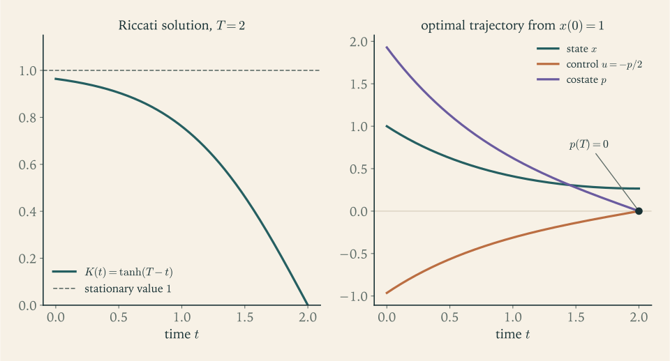
For \(T=2\) and \(x_0=1\) : the optimal cost is \(\tanh2\approx0.9640\) , the initial control is \(u(0)\approx-0.964\) , and the final state is \(x(2)=1/\cosh2\approx0.2658\) . For comparison, the constant-gain feedback \(u=-x\) costs \(1-e^{-4}\approx0.9817\) , and doing nothing costs \(2\) . The gain \(\tanh(T-t)\) is close to \(1\) for most of the interval and falls to \(0\) at the end, where there is no future state cost left for control effort to reduce.
9.4 The linear-quadratic regulator in continuous time
The example is the scalar case of the continuous-time counterpart of Theorem 3.5.
Theorem 9.3 (continuous-time linear-quadratic regulator). Consider \(\dot x=Ax+Bu\) with \(u\in\mathbb R^{m}\) unconstrained and cost \(x(T)^{\top}Q_Tx(T)+\int_0^T(x^{\top}Qx+u^{\top}Ru)\,dt\) , where \(Q\succeq0\) , \(Q_T\succeq0\) , \(R\succ0\) . Suppose the symmetric matrix function \(K(t)\) solves the Riccati differential equation
on \([0,T]\) . Then \(V(t,x)=x^{\top}K(t)x\) , and the optimal control is the linear feedback \(u=-R^{-1}B^{\top}K(t)\,x\) .
Proof. Put \(W(t,x)=x^{\top}K(t)x\) , so that \(W_t=x^{\top}\dot Kx\) and \(\nabla_xW=2Kx\) . The bracket in the Hamilton–Jacobi–Bellman equation is \(x^{\top}Qx+u^{\top}Ru+2x^{\top}K(Ax+Bu)\) , a strictly convex quadratic in \(u\) minimized at \(u=-R^{-1}B^{\top}Kx\) , with minimum value
where \(2x^{\top}KAx\) has been written as \(x^{\top}(A^{\top}K+KA)x\) . By the Riccati equation this equals \(-x^{\top}\dot Kx=-W_t\) . The terminal condition holds because \(K(T)=Q_T\) . The feedback is linear with continuous coefficients, so the closed-loop equation has a solution on \([0,T]\) , and Theorem 9.2 applies.
It can be shown that under the stated sign conditions the Riccati differential equation has a solution on the whole interval \([0,T]\) , so the hypothesis is always met; we do not prove this. As in Chapter 3, when the horizon is long the solution settles, away from the final time, to a constant matrix satisfying the algebraic Riccati equation \(A^{\top}K+KA-KBR^{-1}B^{\top}K+Q=0\) , and under the controllability and observability conditions of Theorem 3.6 the constant feedback \(u=-R^{-1}B^{\top}Kx\) is optimal for the infinite-horizon problem and stabilizes the system.
Example 9.2: The double integrator, with no deadline
Let \(\dot x_1=x_2\) , \(\dot x_2=u\) , with cost \(\int_0^{\infty}(x_1^{2}+u^{2})\,dt\) : position and force are penalized, velocity is not. Here \(A=\begin{pmatrix}0&1\\0&0\end{pmatrix}\) , \(B=\begin{pmatrix}0\\1\end{pmatrix}\) , \(Q=\begin{pmatrix}1&0\\0&0\end{pmatrix}\) , \(R=1\) . Write \(K=\begin{pmatrix}a&b\\b&c\end{pmatrix}\) . Then
and the algebraic Riccati equation gives three scalar equations: \(1-b^{2}=0\) , \(a-bc=0\) , and \(2b-c^{2}=0\) . The positive definite solution has \(b=1\) , \(c=\sqrt2\) , \(a=\sqrt2\) :
The closed-loop matrix \(\begin{pmatrix}0&1\\-1&-\sqrt2\end{pmatrix}\) has eigenvalues \(\tfrac{1}{\sqrt2}(-1\pm i)\) , a well-damped oscillation. From rest at \(x_1=1\) the optimal cost is \(K_{11}=\sqrt2\approx1.414\) .
The Hamilton–Jacobi–Bellman approach has a limitation that these smooth examples hide. Take \(\dot x=u\) with \(\lvert u\rvert\le1\) , no running cost, and terminal cost \(-\lvert x(T)\rvert\) , so that the aim is to end as far from the origin as possible. The best control moves away from the origin at full speed, and \(V(t,x)=-\lvert x\rvert-(T-t)\) . This value function has a corner along \(x=0\) , where two different controls are optimal, and Theorem 9.2 cannot be applied to it. Value functions of problems with bounded controls are often of this kind. A theory of generalized solutions, called viscosity solutions, restores the connection between the equation and the value function; it lies beyond this book.
9.5 Along one trajectory: the costate
The Hamilton–Jacobi–Bellman equation asks for a function on the whole state space, which is out of reach numerically beyond a few dimensions. Pontryagin’s principle asks for much less: conditions along the optimal trajectory alone.
Definition 9.4 (Hamiltonian). The Hamiltonian of the problem of Definition 9.1 is the function
The bracket in the Hamilton–Jacobi–Bellman equation is \(H\) with \(p=\nabla_xV(t,x)\) . The principle keeps the Hamiltonian and replaces the gradient of the unknown value function by a vector \(p(t)\) that satisfies a differential equation of its own.
Theorem 9.5 (Pontryagin’s principle: fixed final time, free final state). Under the standing assumptions of Definition 9.1, with \(U\) an arbitrary subset of \(\mathbb R^{m}\) , let \(u^\star\) be an optimal control with trajectory \(x^\star\) . Then there is a continuous, piecewise continuously differentiable function \(p:[0,T]\to\mathbb R^{n}\) , the costate, such that:
the costate equation holds wherever \(u^\star\) is continuous,
the transversality condition holds at the final time,
and the minimum condition holds at every time \(t\) at which \(u^\star\) is continuous,
If \(H\) is differentiable in \(u\) and \(u^\star(t)\) is an interior point of \(U\) , the minimum condition implies the stationarity condition \(\nabla_uH\big(t,x^\star(t),u^\star(t),p(t)\big)=0\) .
Proof. Define \(p\) as the solution of the costate equation with the terminal value \(p(T)=\nabla\varphi(x^\star(T))\) . The equation is linear in \(p\) with piecewise continuous coefficients, so the solution exists on \([0,T]\) . Only the minimum condition needs proof.
Fix a time \(\tau\in(0,T)\) at which \(u^\star\) is continuous and a point \(v\in U\) . For small \(\varepsilon\) greater than \(0\) let \(u_\varepsilon\) equal \(v\) on the interval \((\tau-\varepsilon,\tau]\) and \(u^\star\) elsewhere, and let \(x_\varepsilon\) be its trajectory. Up to time \(\tau-\varepsilon\) the two trajectories coincide. Over the short interval they separate at the rate \(f(t,x,v)-f(t,x,u^\star)\) , so
After time \(\tau\) both trajectories obey the same differential equation, with control \(u^\star\) , from initial values that differ by \(\varepsilon y(\tau)+o(\varepsilon)\) . Solutions of a differential equation depend differentiably on their initial values, and the derivative is propagated by the linearized equation. Hence for \(t\ge\tau\) , and for \(\varepsilon\) small enough that \(x_\varepsilon\) exists on \([0,T]\) ,
where \(\nabla_xf\) is the Jacobian matrix of \(f\) in \(x\) . The cost changes by the running cost over the short interval, the running cost thereafter, and the terminal cost:
with \(\ell\) and its gradient evaluated along \((x^\star,u^\star)\) . Now compute, using the costate equation \(\dot p=-\nabla_x\ell-(\nabla_xf)^{\top}p\) :
Integrating from \(\tau\) to \(T\) and using \(p(T)=\nabla\varphi(x^\star(T))\) gives \(\int_\tau^T\nabla_x\ell^{\top}y\,dt+\nabla\varphi^{\top}y(T)=p(\tau)^{\top}y(\tau)\) . Therefore
The left side is nonnegative because \(u^\star\) is optimal. Dividing by \(\varepsilon\) and letting \(\varepsilon\to0\) shows that the bracket is nonnegative for every \(v\in U\) , which is the minimum condition at \(\tau\) . The argument took \(\tau\) strictly inside the interval. At \(\tau=0\) or \(\tau=T\) , where the control is continuous from one side, the inequality between the two values of \(H\) follows by letting interior points tend to the endpoint, since \(x^\star\) , \(p\) , and \(u^\star\) are continuous there.
The proof used two facts about differential equations beyond existence and uniqueness: that solutions depend continuously on initial values, so that the perturbed trajectory exists on the whole interval, and that the dependence is differentiable. Both are proved in Differential Equations under the standing assumptions. The perturbation used, a different control on a vanishingly short interval, is called a needle variation. It is large in size and small in duration, which is why no convexity or openness of \(U\) was needed.
The three named conditions each have a job, and it is worth saying what each is. The costate equation runs backward from the final time and carries the information about future costs to the present. Transversality says what the costate is at the end: the marginal cost of the final state. The minimum condition, or stationarity when the minimizer is interior, determines the control from the state and the costate at each instant. Together with the state equation they form a two-point boundary value problem: \(2n\) differential equations for \((x,p)\) , with \(n\) conditions at \(t=0\) , namely \(x(0)=x_0\) , and \(n\) at \(t=T\) , the transversality condition.
The costate is the continuous-time form of a Lagrange multiplier. The state equation is a constraint that must hold at every instant, \(p(t)\)
is the multiplier attached to it at time \(t\)
, and the conditions of the theorem are the analogue of the multiplier conditions for constrained minimization in Continuous Optimization (math.continuous-optimization.kkt-strong-duality). Like a multiplier, the costate measures sensitivity.
Proposition 9.6 (the costate is the gradient of the value function). Suppose the value function \(V\) is twice continuously differentiable and satisfies the Hamilton–Jacobi–Bellman equation, and \(u^\star\) is an optimal control, with trajectory \(x^\star\) , that attains the minimum in that equation along its trajectory. Then \(p(t)=\nabla_xV(t,x^\star(t))\) satisfies the costate equation and the transversality condition of Theorem 9.5.
Proof. Fix \(t\) and consider \(G(x)=V_t(t,x)+\ell(t,x,u^\star(t))+\nabla_xV(t,x)^{\top}f(t,x,u^\star(t))\) . By the Hamilton–Jacobi–Bellman equation \(G(x)\ge0\) for every \(x\) , since the minimum over \(u\) of \(\ell+\nabla_xV^{\top}f\) is \(-V_t\) , and \(G(x^\star(t))=0\) . So \(x^\star(t)\) minimizes \(G\) , and its gradient vanishes there:
On the other hand, differentiating \(p(t)=\nabla_xV(t,x^\star(t))\) along the trajectory gives \(\dot p=\nabla_xV_t+\nabla^{2}_xV\,f\) . Subtracting, \(\dot p=-\nabla_x\ell-(\nabla_xf)^{\top}p=-\nabla_xH\) . At the final time, \(V(T,x)=\varphi(x)\) gives \(p(T)=\nabla\varphi(x^\star(T))\) .
So \(p_i(t)\) is the rate at which the optimal remaining cost would change if the \(i\) -th state component were nudged at time \(t\) . A large costate component marks a state variable whose value matters a great deal to what follows.
Example 9.3: The scalar regulator as a two-point boundary value problem
Return to Example 9.1: \(\dot x=u\) , \(\ell=x^{2}+u^{2}\) , \(\varphi=0\) . The Hamiltonian is \(H=x^{2}+u^{2}+pu\) . The control is unconstrained, so the minimum condition is stationarity: \(H_u=2u+p=0\) , giving \(u=-\tfrac12p\) . The costate equation is \(\dot p=-H_x=-2x\) . Transversality, with no terminal cost, is \(p(T)=0\) . The boundary value problem is
Differentiating, \(\ddot x=x\) , so \(x=\alpha_1\cosh(T-t)+\alpha_2\sinh(T-t)\) and \(p=-2\dot x\) . The condition \(p(T)=0\) gives \(\alpha_2=0\) , and \(x(0)=x_0\) gives
This is the trajectory found in Example 9.1, and \(p(t)=2\tanh(T-t)\,x(t)=V_x(t,x(t))\) , as Proposition 9.6 says.
When no formula is available the boundary value problem is solved numerically. The simplest method is shooting: guess the unknown initial costate \(p(0)\)
, integrate both equations forward to \(T\)
, and adjust the guess until \(p(T)=0\)
. For \(T=2\)
and \(x_0=1\)
the root is \(p(0)\approx1.9281\)
, which is \(2\tanh2\)
, and the integration then gives \(x(1)\approx0.4102\)
, \(p(1)\approx0.6247\)
, and \(x(2)\approx0.2658\)
. Methods for boundary value problems, and the reasons shooting can be ill-conditioned on long intervals, are treated in Numerical Analysis (math.numerical-analysis.boundary-value-synthesis).
Many texts, and most of the aerospace literature, state the principle with a maximum. The translation is mechanical. Put \(\tilde p=-p\) and \(\tilde H(t,x,u,\tilde p)=\tilde p^{\top}f(t,x,u)-\ell(t,x,u)\) , which equals \(-H(t,x,u,p)\) . Then minimizing \(H\) over \(u\) is maximizing \(\tilde H\) ; the costate equation \(\dot p=-\nabla_xH\) becomes \(\dot{\tilde p}=-\nabla_x\tilde H\) , of the same form; and transversality becomes \(\tilde p(T)=-\nabla\varphi(x^\star(T))\) . Before using a formula from another source, check which sign convention it follows.
9.6 Targets, free final time, and the cart
The cart of the opening must arrive at a prescribed state, and its final time is the thing being minimized. Theorem 9.5 covers neither feature. The general statement is as follows.
Theorem 9.7 (Pontryagin’s principle with terminal constraints). In addition to the standing assumptions, let the final state be required to satisfy \(\psi(x(T))=0\) , where \(\psi:\mathbb R^{n}\to\mathbb R^{q}\) is continuously differentiable with a Jacobian matrix \(\nabla\psi\) of rank \(q\) at the final state, and let the final time \(T\) be either fixed or free to be chosen. Assume that there are no constraints on the state along the trajectory, that the control set \(U\) is a fixed set, the same at all times and states, and that \(\varphi\) and \(\psi\) depend on the final state only and not explicitly on the final time. If \(u^\star\) is optimal, with trajectory \(x^\star\) on \([0,T]\) , then there exist a number \(p_0\) equal to \(0\) or \(1\) , a vector \(\nu\in\mathbb R^{q}\) , and a costate \(p(\cdot)\) , with \((p_0,p(t))\ne(0,0)\) for every \(t\) , such that, with the Hamiltonian \(H=p_0\,\ell+p^{\top}f\) :
the costate equation \(\dot p=-\nabla_xH\) and the minimum condition of Theorem 9.5 hold;
the transversality condition reads \(p(T)=p_0\,\nabla\varphi\big(x^\star(T)\big)+\nabla\psi\big(x^\star(T)\big)^{\top}\nu\) ;
if the final time is free, then \(H\big(T,x^\star(T),u^\star(T),p(T)\big)=0\) , where \(u^\star(T)\) is read as the limit of \(u^\star(t)\) as \(t\) increases to \(T\) ;
if \(f\) and \(\ell\) do not depend explicitly on \(t\) , then \(H\big(x^\star(t),u^\star(t),p(t)\big)\) takes the same value at every time \(t\) at which \(u^\star\) is continuous, and that value is \(0\) when the final time is free.
We do not prove this theorem. The proof refines the needle-variation argument: with a terminal constraint the perturbed trajectory must still hit the target, and showing that enough perturbations do so requires a topological argument. The theorem as stated does not cover constraints on the state during the motion, nor a terminal cost or terminal constraint that depends explicitly on the final time; in the latter case the free-time condition is replaced by \(H=-\tfrac{\partial}{\partial T}\big(p_0\varphi+\nu^{\top}\psi\big)\) at the final time. Three remarks make the statement usable.
The transversality condition adapts to the constraint. If the whole final state is prescribed, \(\psi(x)=x-x_T\) , then \(\nabla\psi\) is the identity and the condition says only that \(p(T)\) equals some vector \(\nu\) : it imposes nothing, and the \(n\) missing boundary conditions are supplied by \(x(T)=x_T\) . If only some components of the final state are prescribed, the costate components belonging to the free ones are fixed by \(\nabla\varphi\) . The more the state is pinned at the end, the freer the costate is, and conversely.
The multiplier \(p_0\) . When \(p_0=1\) the problem is called normal and \(H\) is the Hamiltonian of Definition 9.4. The case \(p_0=0\) , called abnormal, occurs when the constraints alone determine the control, so that the cost plays no part in the conditions. With a free final state there is no \(\psi\) , transversality gives \(p(T)=p_0\nabla\varphi\) , and \(p_0=0\) would make \(p\) vanish identically, which is excluded; so Theorem 9.5 is the normal case.
The condition on \(H\) . For a problem that does not depend explicitly on time, the constancy of \(H\) is a useful check on a computed solution, and with free final time \(H\equiv0\) supplies the one extra equation needed to determine \(T\) .
Example 9.4: The minimum-time problem for the double integrator
A cart with position \(x_1\) and velocity \(x_2\) obeys \(\dot x_1=x_2\) , \(\dot x_2=u\) , with \(\lvert u\rvert\le1\) . It is to be brought to rest at the origin, \(x(T)=(0,0)\) , in the least time \(T\) . The cost is \(\int_0^T1\,dt\) , so \(\ell=1\) and \(\varphi=0\) .
The conditions. The Hamiltonian is \(H=p_0+p_1x_2+p_2u\) . The costate equations are \(\dot p_1=-H_{x_1}=0\) and \(\dot p_2=-H_{x_2}=-p_1\) , so
for constants \(c_1,c_2\) . The final state is fully prescribed, so transversality imposes nothing on \(p(T)\) . Minimizing \(H\) over \(u\in[-1,1]\) means minimizing \(p_2u\) :
Could \(p_2\) vanish on an interval? Then \(c_1=c_2=0\) and \(p\equiv0\) ; the free-time condition \(H=0\) would give \(p_0=0\) as well, contradicting \((p_0,p)\ne(0,0)\) . So \(p_2\) is a nonzero linear function of \(t\) , with at most one zero. The optimal control takes only the values \(+1\) and \(-1\) , and switches between them at most once. A control that uses only the extreme values of its range is called bang-bang, and \(p_2\) , whose sign selects the value, is the switching function.
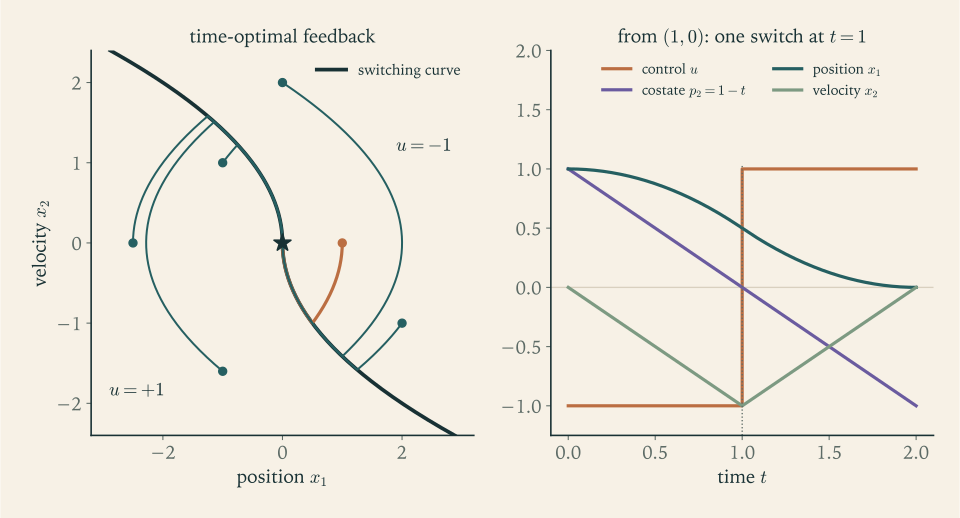
The trajectories. Under \(u=+1\) , \(x_2\) increases at unit rate and \(dx_1/dx_2=x_2\) , so the state moves upward along a parabola \(x_1=\tfrac12x_2^{2}+c\) . Under \(u=-1\) it moves downward along a parabola \(x_1=-\tfrac12x_2^{2}+c\) . Exactly two of these arcs lead into the origin: the lower half of \(x_1=\tfrac12x_2^{2}\) , on which \(u=+1\) and \(x_2\le0\) , and the upper half of \(x_1=-\tfrac12x_2^{2}\) , on which \(u=-1\) and \(x_2\ge0\) . Together they form the switching curve
A trajectory with one switch must make its switch on this curve, since after the switch it must run into the origin without switching again. From a state to the right of the curve the only parabolas that reach the curve are those of \(u=-1\) ; from the left, those of \(u=+1\) . The extremal control is therefore the feedback law: \(u=-1\) if \(x_1+\tfrac12x_2\lvert x_2\rvert\) is positive, \(u=+1\) if it is negative, and on the curve the control that keeps the state on the curve.
The cart at rest one unit from the target. Start at \((1,0)\) , to the right of the curve. With \(u=-1\) : \(x_2=-t\) and \(x_1=1-\tfrac12t^{2}\) . The switching curve is met when \(1-\tfrac12t^{2}=\tfrac12t^{2}\) , at \(t=1\) , in the state \(\big(\tfrac12,-1\big)\) . Then \(u=+1\) for one more unit of time brings the cart to rest at the origin. The time is \(T=2\) .
The costate. The switch at \(t=1\) means \(p_2(1)=0\) , and \(u=-1\) before it means \(p_2\) is positive there: \(p_2(t)=c_1(1-t)\) with \(c_1\) positive. The condition \(H=0\) at \(t=0\) , where \(x_2=0\) and \(u=-1\) , reads \(p_0-c_1=0\) . So \(p_0=1\) , the problem is normal, and
As a check, at time \(t\) in \((1,2)\) , where \(x_2=t-2\) and \(u=1\) , \(H=1+(t-2)+(1-t)=0\) .
Optimality. Pontryagin’s principle is a necessary condition, so it has produced a candidate. For this starting point optimality can be proved directly. Any admissible control gives a velocity \(x_2\) with \(x_2(0)=x_2(T)=0\) and \(\lvert\dot x_2\rvert\le1\) , hence \(\lvert x_2(t)\rvert\le\min\{t,\,T-t\}\) . The cart must cover a distance of \(1\) , so
which gives \(T\ge2\) . The candidate attains \(2\) , so it is optimal.
The minimum time from any state. For a state to the right of the switching curve, following \(u=-1\) to the curve and then \(u=+1\) to the origin takes
and for a state to the left, \(T=-x_2+2\sqrt{-x_1+\tfrac12x_2^{2}}\) . At \((1,0)\) this gives \(2\) . Its gradient at \((1,0)\) is \((1,1)\) , which is the costate \((p_1(0),p_2(0))\) found above, in agreement with Proposition 9.6. The function \(T(x)\) is not differentiable across the switching curve: it is one more value function with a crease.
9.7 Fuel, and the arc on which the engine is off
If what is scarce is fuel and not time, the cost is the total control effort \(\int\lvert u\rvert\,dt\) . The Hamiltonian is then not differentiable in \(u\) , and stationarity is not available, but the minimum condition is, and it produces a third kind of arc.
Example 9.5: Minimum fuel with a fixed transfer time
Move the same cart from rest at \(x_1=1\) to rest at the origin in a fixed time \(T=3\) , which is longer than the minimum time of \(2\) , using the least fuel \(\int_0^3\lvert u\rvert\,dt\) , with \(\lvert u\rvert\le1\) .
The Hamiltonian, in the normal case, is \(H=\lvert u\rvert+p_1x_2+p_2u\) , and the costate is as before: \(p_1=c_1\) , \(p_2=c_2-c_1t\) . Minimize \(\lvert u\rvert+p_2u\) over \(u\in[-1,1]\) . For \(u\ge0\) the expression is \((1+p_2)\,u\) , which is smallest at \(u=0\) unless \(p_2\) is below \(-1\) , when it is smallest at \(u=1\) . For \(u\le0\) it is \((1-p_2)\,\lvert u\rvert\) , which is smallest at \(u=0\) unless \(p_2\) exceeds \(1\) , when it is smallest at \(u=-1\) . So
Using the engine is worthwhile only when the costate of velocity outweighs the unit price of fuel. Since \(p_2\) is linear in \(t\) , the control passes through the values \(-1\) , \(0\) , \(+1\) in that order or its reverse, each at most once: bang-off-bang.
By symmetry try \(u=-1\) on \([0,t_1]\) , \(u=0\) on \((t_1,3-t_1)\) , and \(u=+1\) on \([3-t_1,3]\) . The velocity falls to \(-t_1\) , stays there during the coast, and returns to \(0\) . The distance covered is \(\tfrac12t_1^{2}+t_1(3-2t_1)+\tfrac12t_1^{2}=t_1(3-t_1)\) , which must equal \(1\) :
The fuel used is \(2t_1=3-\sqrt5\approx0.764\) , against \(2\) for the minimum-time transfer. The costate that produces these switch times is the linear function with \(p_2(t_1)=1\) and \(p_2(3-t_1)=-1\) :
since \(3-2t_1=\sqrt5\) . It starts at \(p_2(0)\approx1.342\) , above \(1\) , and ends at \(-1.342\) , as the control sequence requires.
For a general transfer time \(T\ge2\) the same computation gives \(t_1=\tfrac12\big(T-\sqrt{T^{2}-4}\big)\) and fuel \(T-\sqrt{T^{2}-4}\) : \(2\) at \(T=2\) , \(0.764\) at \(T=3\) , \(0.417\) at \(T=5\) , and about \(2/T\) for large \(T\) . Allowing a little more time saves a great deal of fuel, and the saving is taken as a coasting arc in the middle. This is the pattern of impulsive burns separated by coasts that governs the transfer of spacecraft between orbits. Theorem 9.8 below shows that the candidate is optimal.
9.8 Necessary is not sufficient
Example 9.6: An extremal that is the worst control
Let \(\dot x=u\) with \(\lvert u\rvert\le1\) , \(x(0)=0\) , final time \(1\) , no running cost, and terminal cost \(\varphi(x)=-x^{2}\) . The Hamiltonian is \(H=pu\) , the costate equation is \(\dot p=0\) , and transversality gives \(p=-2x(1)\) , a constant. The minimum condition gives \(u=-\operatorname{sgn}p\) when \(p\ne0\) .
Three controls satisfy all the conditions. With \(u\equiv1\) : \(x(1)=1\) and \(p=-2\) , and \(u=-\operatorname{sgn}p=1\) . With \(u\equiv-1\) : \(x(1)=-1\) , \(p=2\) , \(u=-1\) . With \(u\equiv0\) : \(x(1)=0\) and \(p=0\) , so that \(H\equiv0\) for every \(u\) and the minimum condition holds trivially. The first two have cost \(-1\) and are optimal. The third has cost \(0\) , which is the largest cost any admissible control can have.
A control satisfying Pontryagin’s conditions is called an extremal. The example shows that an extremal need not be optimal, or even locally optimal. The conditions are the dynamic analogue of a vanishing derivative, which holds at maxima and saddle points as well as at minima. As in static optimization, convexity is what closes the gap.
Theorem 9.8 (sufficiency under convexity). Consider the problem of Definition 9.1 with fixed final time and either a free final state or a prescribed final state \(x(T)=x_T\) . Let \(u^\star\) be admissible with trajectory \(x^\star\) , and let \(p(\cdot)\) satisfy the costate equation along it, together with \(p(T)=\nabla\varphi(x^\star(T))\) in the free case. Suppose \(\varphi\) is convex, and that for every \(t\) , every \(x\in\mathbb R^{n}\) , and every \(u\in U\) ,
Then \(u^\star\) is optimal. The displayed inequality holds, in particular, when \(U\) is convex, the function \((x,u)\mapsto H(t,x,u,p(t))\) is convex and differentiable, and \(u^\star(t)\) satisfies the minimum condition; and also when \(H\) is the sum of a function affine in \(x\) and a function of \(u\) alone that \(u^\star(t)\) minimizes over \(U\) .
Proof. Let \(u\) be admissible with trajectory \(x\) satisfying the same end conditions, and write \(\Delta(t)=x(t)-x^\star(t)\) , so that \(\Delta(0)=0\) . Since \(\ell=H-p^{\top}f\) and \(\dot x=f\) along each trajectory,
By the hypothesis and the costate equation, \(H(t,x,u,p)-H(t,x^\star,u^\star,p)\ge\nabla_xH^{\top}\Delta=-\dot p^{\top}\Delta\) , so the integrand is at least \(-\dot p^{\top}\Delta-p^{\top}\dot\Delta=-\tfrac{d}{dt}(p^{\top}\Delta)\) , and the integral is at least \(-p(T)^{\top}\Delta(T)\) . By convexity of \(\varphi\) , the terminal difference is at least \(\nabla\varphi(x^\star(T))^{\top}\Delta(T)\) . Hence
which is \(0\) in the free case by transversality and \(0\) in the prescribed case because \(\Delta(T)=0\) , the terminal cost then being the same constant for both.
For the first special case, convexity and differentiability give \(H(x,u)-H(x^\star,u^\star)\ge\nabla_xH^{\top}(x-x^\star)+\nabla_uH^{\top}(u-u^\star)\) , and the last term is nonnegative because \(u^\star\) minimizes the convex function \(H(t,x^\star,\cdot,p)\) over the convex set \(U\) . For the second, the affine part contributes exactly \(\nabla_xH^{\top}(x-x^\star)\) and the remaining part is nonnegative by the minimum condition.
The theorem settles the earlier examples. In Example 9.3 the Hamiltonian \(x^{2}+u^{2}+pu\) is convex in \((x,u)\) , so the solution of the boundary value problem is optimal, with no appeal to the Hamilton–Jacobi–Bellman equation. In Example 9.5 the Hamiltonian is \(p_1x_2\) , which is affine in \(x\) , plus \(\lvert u\rvert+p_2u\) , which \(u^\star\) minimizes; so the bang-off-bang control is optimal. In Example 9.6 the terminal cost \(-x^{2}\) is concave, and the theorem is silent, as it must be.
The two approaches of this chapter can now be set side by side.
| Hamilton–Jacobi–Bellman | Pontryagin | |
|---|---|---|
| Unknown | a function \(V(t,x)\) on the whole state space | functions \(x(t)\) , \(p(t)\) along one trajectory |
| Equation | one partial differential equation | \(2n\) ordinary differential equations with conditions at both ends |
| Logical status | sufficient, given a smooth solution | necessary; sufficient under convexity |
| Output | a feedback law for every state | an open-loop control from one initial state |
| Main obstacle | dimension of the state; value functions with creases | several extremals; sensitive boundary value problems |
In low dimensions, or when a formula such as the quadratic one is available, the first is preferable because it yields feedback. In high dimensions, as in trajectory design, only the second is practical. Chapter 10 takes up a third course that borrows from both: solve an open-loop problem over a short horizon, apply the start of its solution, and repeat from the state that results.
Exercises
-
For the problem of Definition 9.1 write the Hamilton–Jacobi–Bellman equation with its terminal condition, and write the Hamiltonian together with the costate equation, the minimum condition, the stationarity condition, and the transversality condition of Theorem 9.5, saying in one phrase what each of the last four determines.
Hint
The Hamilton–Jacobi–Bellman equation is \(-V_t=\min_{u\in U}[\ell+\nabla_xV^{\top}f]\) with \(V(T,x)=\varphi(x)\) . With \(H=\ell+p^{\top}f\) : the costate equation \(\dot p=-\nabla_xH\) determines how \(p\) evolves; the minimum condition determines the control from \(x\) and \(p\) ; stationarity, \(\nabla_uH=0\) , is its form when the minimizer is interior; transversality, \(p(T)=\nabla\varphi(x(T))\) , supplies the boundary condition for \(p\) .
-
Let \(\dot x=u\) with \(u\) unconstrained and cost \(x(T)^{2}+\int_0^Tu^{2}\,dt\) . Solve the Hamilton–Jacobi–Bellman equation with the trial form \(V=K(t)x^{2}\) , and give the optimal feedback, the optimal trajectory from \(x_0\) , and the optimal cost.
Solution
The equation is \(-V_t=\min_u[u^{2}+V_xu]\) , with \(V(T,x)=x^{2}\) . The bracket is minimized at \(u=-\tfrac12V_x\) , with minimum \(-\tfrac14V_x^{2}\) . Try \(V=K(t)x^{2}\) : then \(V_t=\dot Kx^{2}\) , \(V_x=2Kx\) , and the equation becomes \(-\dot Kx^{2}=-K^{2}x^{2}\) , that is,
\[ \dot K=K^{2},\qquad K(T)=1 . \]Separating variables, \(-\dfrac1K=t+c\) , and the terminal condition gives \(c=-(1+T)\) , so
\[ K(t)=\frac{1}{1+T-t}. \]This is continuously differentiable on \([0,T]\) , so by Theorem 9.2 it gives the value function \(V=\dfrac{x^{2}}{1+T-t}\) and the optimal feedback \(u=-Kx=-\dfrac{x}{1+T-t}\) .
The closed loop \(\dot x=-\dfrac{x}{1+T-t}\) has the solution \(x(t)=x_0\,\dfrac{1+T-t}{1+T}\) , a straight line in \(t\) , so the control is constant: \(u=-\dfrac{x_0}{1+T}\) . The optimal cost is \(V(0,x_0)=\dfrac{x_0^{2}}{1+T}\) . As a check, \(x(T)=\dfrac{x_0}{1+T}\) , so the terminal cost is \(\dfrac{x_0^{2}}{(1+T)^{2}}\) and the control cost is \(T\,\dfrac{x_0^{2}}{(1+T)^{2}}\) , which add to \(\dfrac{x_0^{2}}{1+T}\) .
-
Solve the problem of Exercise 2 by Pontryagin’s principle: write the Hamiltonian, the stationarity and costate equations, and the transversality condition, solve the boundary value problem, and check that the answer agrees with Exercise 2.
Solution
The Hamiltonian is \(H=u^{2}+pu\) , since \(\ell=u^{2}\) and \(f=u\) . Stationarity: \(H_u=2u+p=0\) , so \(u=-\tfrac12p\) . Costate equation: \(\dot p=-H_x=0\) , so \(p\) is constant. Transversality: \(p(T)=\varphi'(x(T))=2x(T)\) .
So \(u\) is the constant \(-\tfrac12p=-x(T)\) , and the state is \(x(t)=x_0-x(T)\,t\) . Setting \(t=T\) : \(x(T)=x_0-T\,x(T)\) , hence
\[ x(T)=\frac{x_0}{1+T},\qquad u\equiv-\frac{x_0}{1+T},\qquad p\equiv\frac{2x_0}{1+T}. \]This is the control found in Exercise 2. The costate also agrees with Proposition 9.6: \(V_x(t,x(t))=\dfrac{2x(t)}{1+T-t}=\dfrac{2x_0}{1+T}\) for every \(t\) .
The Hamiltonian \(u^{2}+pu\) is convex in \((x,u)\) and the terminal cost \(x^{2}\) is convex, so by Theorem 9.8 the extremal is optimal; the boundary value problem alone settles the question. The unknown constant \(p\) was found from a condition at the final time, which is typical: the costate is pinned at the end, the state at the beginning.
-
For the unstable scalar system \(\dot x=x+u\) with cost \(\int_0^{\infty}(x^{2}+u^{2})\,dt\) , solve the algebraic Riccati equation, give the optimal feedback, and find the closed-loop dynamics.
Solution
Here \(A=1\) , \(B=1\) , \(Q=1\) , \(R=1\) , and the algebraic Riccati equation \(A^{\top}K+KA-KBR^{-1}B^{\top}K+Q=0\) is the scalar equation \(2K-K^{2}+1=0\) . Its roots are \(1\pm\sqrt2\) , and the positive one is \(K=1+\sqrt2\approx2.414\) .
The optimal feedback is \(u=-R^{-1}B^{\top}Kx=-(1+\sqrt2)\,x\) , and the closed loop is \(\dot x=x-(1+\sqrt2)x\) , that is, \(\dot x=-\sqrt2\,x\) . The optimal cost from \(x_0\) is \((1+\sqrt2)\,x_0^{2}\) .
The open loop \(\dot x=x\) is unstable, with growth rate \(1\) ; the closed loop is stable, with decay rate \(\sqrt2\) . The negative root \(1-\sqrt2\) also solves the equation, but it would give the feedback \(u=(\sqrt2-1)x\) and the closed loop \(\dot x=\sqrt2\,x\) , which is unstable with infinite cost. Among the solutions of the algebraic equation, the one that corresponds to the regulator is the positive semidefinite, stabilizing one.
-
Verify by differentiation that \(K(t)=\tanh(T-t)\) solves \(\dot K=K^{2}-1\) with \(K(T)=0\) . Then show that with the terminal cost \(x(T)^{2}\) added to the problem of Example 9.1 the solution of the Riccati equation is \(K(t)=1\) for all \(t\) , and interpret the result.
Answer
\(\dfrac{d}{dt}\tanh(T-t)=-\big(1-\tanh^{2}(T-t)\big)=K^{2}-1\) , and \(\tanh0=0\) . With terminal cost \(x(T)^{2}\) the condition is \(K(T)=1\) , and the constant \(K\equiv1\) satisfies \(\dot K=K^{2}-1=0\) . The optimal feedback is then \(u=-x\) at all times: the terminal cost \(x^{2}\) is exactly the cost of continuing optimally for ever, so the finite-horizon problem looks, at every instant, like the infinite-horizon one.
-
In the proof of Theorem 9.2 the function \(t\mapsto W(t,x(t))\) is differentiated on intervals where the control is continuous. Explain why the conclusion survives finitely many points of discontinuity of the control, stating which property of \(W(t,x(t))\) as a function of \(t\) is used.
Hint
The state \(x(t)\) is continuous even where the control jumps, so \(t\mapsto W(t,x(t))\) is continuous on \([0,T]\) and differentiable except at finitely many points. For such a function the total change is the sum of the integrals of its derivative over the pieces. Continuity is what makes the pieces join without gaps.
-
For the minimum-time problem of Example 9.4, find the optimal control, the switching time and state, and the minimum time from the initial state \((x_1,x_2)=(0,2)\) , a cart passing through the target at speed \(2\) .
Solution
At \((0,2)\) the quantity \(x_1+\tfrac12x_2\lvert x_2\rvert=2\) is positive, so the state is to the right of the switching curve and the control starts at \(u=-1\) .
First arc. With \(u=-1\) from \((0,2)\) : \(x_2=2-t\) and \(x_1=2t-\tfrac12t^{2}\) . The cart continues past the target, slows, stops at \(t=2\) with \(x_1=2\) , and starts back.
Switch. The arc into the origin with \(u=+1\) is \(x_1=\tfrac12x_2^{2}\) with \(x_2\le0\) . The first arc meets it when \(2t-\tfrac12t^{2}=\tfrac12(2-t)^{2}\) , that is, \(t^{2}-4t+2=0\) , so \(t=2\pm\sqrt2\) . The velocity must be negative, which selects \(t_s=2+\sqrt2\approx3.414\) . The state there is \(\big(1,-\sqrt2\big)\) .
Second arc. With \(u=+1\) the velocity rises from \(-\sqrt2\) to \(0\) in time \(\sqrt2\) , and the cart arrives at rest at the origin.
The minimum time is \(T=2+2\sqrt2\approx4.828\) , in agreement with the formula \(x_2+2\sqrt{x_1+\tfrac12x_2^{2}}=2+2\sqrt2\) . The cart is at the target at the outset, but moving too fast to stop there; it must overshoot by two units, and the optimal control brakes at full force from the start.
-
For a state to the right of the switching curve in Example 9.4, derive the formula \(T(x_1,x_2)=x_2+2\sqrt{x_1+\tfrac12x_2^{2}}\) , and verify that it satisfies the stationary Hamilton–Jacobi–Bellman equation \(\min_{\lvert u\rvert\le1}\big[1+T_{x_1}x_2+T_{x_2}u\big]=0\) in that region.
Solution
Derivation. From \((x_1,x_2)\) to the right of the curve apply \(u=-1\) for a time \(\tau\) , reaching velocity \(x_2-\tau\) and position \(x_1+x_2\tau-\tfrac12\tau^{2}\) . This point is on the arc \(x_1=\tfrac12x_2^{2}\) when \(x_1+x_2\tau-\tfrac12\tau^{2}=\tfrac12(x_2-\tau)^{2}\) , that is, \(\tau^{2}-2x_2\tau-\big(x_1-\tfrac12x_2^{2}\big)=0\) , with root \(\tau=x_2+s\) , where \(s=\sqrt{x_1+\tfrac12x_2^{2}}\) ; the other root would give a positive velocity at the switch. The velocity at the switch is \(-s\) , and the second arc takes time \(s\) . So \(T=x_2+2s\) .
Verification. \(T_{x_1}=\dfrac1s\) and \(T_{x_2}=1+\dfrac{x_2}{s}\) . To the right of the curve \(T_{x_2}\) is positive: for \(x_2\ge0\) this is clear, and for negative \(x_2\) it says \(s>\lvert x_2\rvert\) , that is, \(x_1>\tfrac12x_2^{2}\) , which is the condition of lying to the right of the lower arc. So the minimizing control is \(u=-1\) , and
\[ 1+T_{x_1}x_2+T_{x_2}u=1+\frac{x_2}{s}-\Big(1+\frac{x_2}{s}\Big)=0 . \]The equation holds in the region, with \(u=-1\) as the minimizer, in agreement with the feedback law of Example 9.4. On the switching curve itself \(T\) is not differentiable, and the equation cannot be interpreted there in the ordinary sense.
-
A student writes: “The control \(u\equiv0\) in Example 9.6 satisfies the costate equation, transversality, and the minimum condition, so by Pontryagin’s principle it is optimal.” State what Pontryagin’s principle asserts and what it does not, and name a hypothesis of Theorem 9.8 that fails in that example.
Answer
The principle asserts that an optimal control satisfies the conditions. It does not assert the converse. The control \(u\equiv0\) is an extremal with cost \(0\) , the worst possible. Theorem 9.8 does not rescue the argument, because the terminal cost \(-x^{2}\) is not convex.
-
A student solves Exercise 3 using the transversality condition \(p(T)=0\) , “because the final state is free”. Find the control this produces and its cost from \(x_0\) , compare with the optimal cost, and state the correct transversality condition and why it differs.
Solution
With \(p(T)=0\) and \(\dot p=0\) the costate is identically zero, stationarity gives \(u=-\tfrac12p\equiv0\) , and the state stays at \(x_0\) . The cost is the terminal cost \(x_0^{2}\) , with no control cost.
The optimal cost, from Exercise 2, is \(\dfrac{x_0^{2}}{1+T}\) . For \(T=1\) the student’s control costs twice the optimum, and the ratio grows with \(T\) .
The correct condition is \(p(T)=\nabla\varphi(x(T))=2x(T)\) . “Free final state” means that no constraint is imposed on \(x(T)\) ; it does not mean that the final state is free of cost. Transversality equates the costate at the final time with the marginal terminal cost. Only when there is no terminal cost, as in Example 9.3, does this reduce to \(p(T)=0\) . The student’s condition describes a different problem, the one with \(\varphi=0\) , in which doing nothing is indeed optimal.
-
For the minimum-fuel problem of Example 9.5 with transfer time \(T=4\) , find the switch times, the fuel used, and the costate \(p_2(t)\) . Then show that the fuel \(T-\sqrt{T^{2}-4}\) behaves like \(2/T\) for large \(T\) .
Solution
For transfer time \(T\) the switch time satisfies \(t_1(T-t_1)=1\) . With \(T=4\) : \(t_1^{2}-4t_1+1=0\) , so \(t_1=2-\sqrt3\approx0.268\) , taking the root less than \(T/2\) . The control is \(-1\) on \([0,\,0.268]\) , zero on \((0.268,\,3.732)\) , and \(+1\) on \([3.732,\,4]\) . The fuel is \(2t_1=4-2\sqrt3\approx0.536\) .
The costate \(p_2\) is linear with \(p_2(t_1)=1\) and \(p_2(T-t_1)=-1\) . The coast lasts \(T-2t_1=2\sqrt3\) , so
\[ p_2(t)=1-\frac{2\,(t-t_1)}{2\sqrt3}=1-\frac{t-t_1}{\sqrt3},\qquad p_1=\frac1{\sqrt3}. \]For large \(T\) , multiply and divide by the conjugate: \(T-\sqrt{T^{2}-4}=\dfrac{4}{T+\sqrt{T^{2}-4}}\) , and the denominator is close to \(2T\) , so the fuel is close to \(\dfrac2T\) . With a long time available the cart is given a small velocity of about \(1/T\) by a short burn, coasts nearly the whole way, and is stopped by an equal burn; the fuel is twice that velocity.
-
Move the cart of Example 9.4 from rest at \(x_1=1\) to rest at the origin in a fixed time \(T\) with unconstrained control, minimizing the energy \(\int_0^Tu^{2}\,dt\) . Use Pontryagin’s principle to show that the optimal control is linear in \(t\) , find it, and compute the minimum energy. For \(T=2\) compare the peak force and the energy with those of the bang-bang control.
Solution
The Hamiltonian is \(H=u^{2}+p_1x_2+p_2u\) . Stationarity gives \(2u+p_2=0\) , and the costate equations \(\dot p_1=0\) , \(\dot p_2=-p_1\) make \(p_2\) linear in \(t\) . So \(u(t)=a+bt\) for constants \(a\) , \(b\) , which the end conditions determine; the final state is prescribed, so transversality imposes nothing.
Velocity: \(x_2(t)=at+\tfrac12bt^{2}\) , and \(x_2(T)=0\) gives \(a=-\tfrac12bT\) . Position: \(x_1(T)=1+\tfrac12aT^{2}+\tfrac16bT^{3}=1-\tfrac1{12}bT^{3}\) , and \(x_1(T)=0\) gives \(b=\dfrac{12}{T^{3}}\) , \(a=-\dfrac{6}{T^{2}}\) :
\[ u(t)=-\frac{6}{T^{2}}+\frac{12\,t}{T^{3}} . \]The control starts at \(-\tfrac{6}{T^{2}}\) , passes through zero at the midpoint, and ends at \(+\tfrac{6}{T^{2}}\) . The energy is \(\int_0^T(a+bt)^{2}dt\) ; with \(s=t-\tfrac T2\) this is \(\int_{-T/2}^{T/2}b^{2}s^{2}\,ds=\dfrac{b^{2}T^{3}}{12}\) , which equals \(\dfrac{12}{T^{3}}\) .
By Theorem 9.8 the control is optimal, since \(H\) is convex in \((x,u)\) . For \(T=2\) the energy is \(1.5\) and the peak force is \(1.5\) . The bang-bang control of Example 9.4 has energy \(\int_0^21\,dt=2\) and peak force \(1\) . The minimum-energy control is cheaper in energy but needs a force that the constrained cart cannot supply; with the bound \(\lvert u\rvert\le1\) and \(T=2\) the bang-bang control is the only admissible one.
-
Let \(f\) and \(\ell\) not depend explicitly on \(t\) , let \(U=\mathbb R^{m}\) , and let \((x,u,p)\) be smooth functions of \(t\) satisfying the state equation, the costate equation, and stationarity. Prove that \(H(x(t),u(t),p(t))\) is constant.
Hint
Differentiate \(H(x(t),u(t),p(t))\) by the chain rule: \(\dot H=\nabla_xH^{\top}\dot x+\nabla_uH^{\top}\dot u+\nabla_pH^{\top}\dot p\) . Use \(\nabla_pH=f=\dot x\) , the costate equation \(\dot p=-\nabla_xH\) , and stationarity \(\nabla_uH=0\) . The first and third terms cancel and the second vanishes.
-
For Example 9.1 with \(T=2\) , estimate the derivative of the optimal cost with respect to the initial state at \(x_0=1\) by comparing the costs from \(x_0=1\) and \(x_0=1.01\) , and compare the estimate with \(p(0)\) from Example 9.3.
Answer
The optimal cost is \(\tanh(2)\,x_0^{2}\) : \(0.96403\) at \(x_0=1\) and \(0.98340\) at \(x_0=1.01\) . The difference quotient is \(1.938\) . The costate is \(p(0)=2\tanh2\approx1.928\) , the exact derivative; the quotient differs by the second-order term \(\tanh(2)\cdot0.01\) .
-
Discretize the problem of Example 9.1 with step \(h\) : \(x_{k+1}=x_k+hu_k\) and stage cost \(h\,(x_k^{2}+u_k^{2})\) . Show from Exercise 3.11 that the Riccati recursion is \(K_k=h+\dfrac{K_{k+1}}{1+hK_{k+1}}\) , that \(\dfrac{K_k-K_{k+1}}{h}\to1-K^{2}\) as \(h\to0\) , and compute \(K_0\) for \(T=1\) with \(h=0.1\) for comparison with \(\tanh1\) .
Solution
In the notation of Exercise 3.11 the discretized problem has \(a=1\) , \(b=h\) , \(q=h\) , \(r=h\) . The recursion \(K_k=q+\dfrac{a^{2}rK_{k+1}}{r+b^{2}K_{k+1}}\) becomes
\[ K_k=h+\frac{hK_{k+1}}{h+h^{2}K_{k+1}}=h+\frac{K_{k+1}}{1+hK_{k+1}} . \]Writing \(K\) for \(K_{k+1}\) ,
\[ \frac{K_k-K_{k+1}}{h}=1+\frac1h\Big(\frac{K}{1+hK}-K\Big)=1-\frac{K^{2}}{1+hK}\ \longrightarrow\ 1-K^{2}\qquad(h\to0). \]Since \(K_k\) belongs to the earlier time, the left side approximates \(-\dot K\) , and the limit is the Riccati differential equation \(\dot K=K^{2}-1\) of Example 9.1. The terminal condition \(K_N=0\) matches \(K(T)=0\) .
For \(T=1\) and \(h=0.1\) , ten backward steps from \(K_{10}=0\) give \(K_0\approx0.7905\) , against \(\tanh1\approx0.7616\) . The discrete value is larger because a control held constant over each step is less effective than a continuously adjusted one. The error is roughly proportional to \(h\) : with \(h=0.01\) the recursion gives \(0.7645\) .
-
Restate Theorem 9.5 in maximum form, with \(\tilde p=-p\) and \(\tilde H=\tilde p^{\top}f-\ell\) : give the costate equation, the transversality condition, and the condition on the control, and apply the restated theorem to Example 9.3 to confirm that it yields the same control.
Answer
With \(\tilde H=\tilde p^{\top}f-\ell\) : the costate equation is \(\dot{\tilde p}=-\nabla_x\tilde H\) ; transversality is \(\tilde p(T)=-\nabla\varphi(x^\star(T))\) ; and \(u^\star(t)\) maximizes \(\tilde H(t,x^\star(t),v,\tilde p(t))\) over \(v\in U\) . For Example 9.3, \(\tilde H=\tilde pu-x^{2}-u^{2}\) , maximized at \(u=\tfrac12\tilde p\) ; \(\dot{\tilde p}=2x\) ; \(\tilde p(T)=0\) . With \(\tilde p=-p\) these are the equations of that example, and \(u=\tfrac12\tilde p=-\tfrac12p\) .
-
Let \(\dot x=u\) with \(\lvert u\rvert\le1\) , \(x(0)=1\) , final time \(2\) , and cost \(\int_0^2x^{2}\,dt\) . Show that the control equal to \(-1\) on \([0,1]\) and \(0\) on \((1,2]\) satisfies the conditions of Theorem 9.5 with \(p(t)=(1-t)^{2}\) on \([0,1]\) and \(p(t)=0\) afterwards, explain why the minimum condition does not determine the control on \((1,2]\) , and prove the control optimal.
Solution
The candidate. On \([0,1]\) , \(u=-1\) gives \(x(t)=1-t\) ; on \((1,2]\) , \(u=0\) keeps \(x=0\) .
Costate. The Hamiltonian is \(H=x^{2}+pu\) , so \(\dot p=-2x\) , with \(p(2)=0\) since there is no terminal cost. On \((1,2]\) , \(x=0\) gives \(\dot p=0\) and \(p=0\) . On \([0,1]\) , \(\dot p=-2(1-t)\) with \(p(1)=0\) gives \(p(t)=(1-t)^{2}\) , and indeed \(\tfrac{d}{dt}(1-t)^{2}=-2(1-t)\) .
Minimum condition. \(H\) depends on \(u\) through \(pu\) . On \([0,1)\) , \(p\) is positive, so the minimum over \([-1,1]\) is at \(u=-1\) , as used. On \((1,2]\) , \(p=0\) and \(H\) does not depend on \(u\) at all: every \(u\) minimizes, and the condition gives no information. Such an arc is called singular. The control there is determined by the requirement that \(p\) remain zero, which through \(\dot p=-2x\) forces \(x=0\) and hence \(u=0\) .
Optimality. \(U=[-1,1]\) is convex and \(H=x^{2}+pu\) is convex and differentiable in \((x,u)\) ; the candidate satisfies the costate equation, transversality, and the minimum condition. By Theorem 9.8 it is optimal. Its cost is \(\int_0^1(1-t)^{2}\,dt=\tfrac13\) . A direct argument agrees: \(x\) can decrease no faster than at unit rate, so \(x(t)\ge1-t\) on \([0,1]\) and \(x(t)^{2}\ge0\) afterwards.
-
For the scalar system \(\dot x=-x+u\) with \(\lvert u\rvert\le1\) , find the control that brings \(x(0)=x_0\) , with \(x_0\) positive, to the origin in minimum time, and the minimum time, and show from the costate equation that the optimal control never switches.
Answer
\(u=-1\) throughout. Then \(\dot x=-x-1\) , so \(x(t)=(x_0+1)e^{-t}-1\) , which reaches \(0\) at \(T=\log(1+x_0)\) . The Hamiltonian is \(p_0+p\,(-x+u)\) , the costate equation is \(\dot p=p\) , so \(p(t)=p(0)e^{t}\) never changes sign, and \(u=-\operatorname{sgn}p\) never switches. For positive \(x_0\) the sign must be the one giving \(u=-1\) .
-
Let \(\dot x=u\) with \(\lvert u\rvert\le1\) and cost \(x(T)^{2}\) . Show that \(W(t,x)=\big(\max\{\lvert x\rvert-(T-t),\,0\}\big)^{2}\) is continuously differentiable and satisfies the Hamilton–Jacobi–Bellman equation with its terminal condition, and state the optimal feedback.
Solution
Write \(d(t,x)=\lvert x\rvert-(T-t)\) , so \(W=\big(\max\{d,0\}\big)^{2}\) .
Smoothness. The function \(m\mapsto(\max\{m,0\})^{2}\) is continuously differentiable, with derivative \(2\max\{m,0\}\) . Away from \(x=0\) , \(d\) is differentiable, so \(W\) is continuously differentiable there, with \(W_t=2\max\{d,0\}\) and \(W_x=2\max\{d,0\}\operatorname{sgn}x\) . Near \(x=0\) with \(t\) less than \(T\) , \(d\) is negative and \(W\) vanishes identically. At \(t=T\) , \(W=x^{2}\) , which is smooth. So \(W\) is continuously differentiable on \([0,T]\times\mathbb R\) .
The equation. Here \(\ell=0\) and \(f=u\) , so the equation is \(-W_t=\min_{\lvert u\rvert\le1}W_xu=-\lvert W_x\rvert\) . Where \(d\) is positive, \(W_t=2d\) and \(\lvert W_x\rvert=2d\) , so both sides equal \(-2d\) . Where \(d\le0\) , both sides are \(0\) . The terminal condition is \(W(T,x)=(\max\{\lvert x\rvert,0\})^{2}=x^{2}\) .
Feedback. The minimizing control is \(u=-\operatorname{sgn}x\) where \(d\) is positive: drive toward the origin at full speed. Where \(d\le0\) the origin can be reached in the time remaining, \(W_x=0\) , and any control that keeps \(\lvert x\rvert\le T-t\) and ends at \(x(T)=0\) is optimal, for example \(u=-\operatorname{sgn}x\) until the origin is reached and \(0\) afterwards. By Theorem 9.2, \(W\) is the value function: the optimal cost is the square of the distance by which the origin cannot be reached.
-
Using the formula of Example 9.5, tabulate the minimum fuel for transfer times \(T=2,3,5,10\) for the rest-to-rest transfer over unit distance, and describe how the optimal control changes as \(T\) increases.
Answer
Fuel \(T-\sqrt{T^{2}-4}\) : \(2\) at \(T=2\) ; \(0.764\) at \(T=3\) ; \(0.417\) at \(T=5\) ; \(0.202\) at \(T=10\) . At \(T=2\) the control is bang-bang with no coast. As \(T\) increases the two burns shrink toward the ends of the interval, each of length about \(1/T\) , and the coast fills the rest.