Someone has a house to sell and a week in which to sell it. One offer arrives each day. An offer that is declined is gone; the last one must be taken. Monday’s offer is decent. Accept it, or wait for a better one that may never come?
Problems of this kind have the simplest possible control set, stop or continue, and they are everywhere: when to sell, when to exercise an option, when to stop testing and decide, when to replace, when to hire. The Bellman recursion applies to them without change. What makes them a subject of their own is the form the answer takes. In problem after problem the optimal policy is a threshold rule: stop when some quantity crosses a level. This chapter shows where thresholds come from, how to compute them, how they move with the time remaining, and when a much cheaper rule, which looks only one step ahead, is already optimal.
Stopping problems are usually posed with rewards, and in this chapter the recursions maximize.
8.1 Stop or continue
Definition 8.1 (optimal stopping problem). A state \(x_k\) evolves as a Markov chain with given transition probabilities, not influenced by the decision maker, for stages \(k=0,\dots,N\) . At each stage \(k\) the decision maker observes \(x_k\) and either stops, receiving a reward \(t_k(x_k)\) and ending the problem, or continues, receiving \(c_k(x_k)\) and moving to stage \(k+1\) . At stage \(N\) stopping is compulsory. The objective is to maximize the expected total reward.
This is a model in the sense of Definition 1.1 once a “stopped” state is added, which is entered on stopping and never left and in which nothing more is earned; Exercise 12 asks for the details. Theorem 2.2 then gives
and it is optimal to stop at stage \(k\) exactly when the first term attains the maximum. The set
is the stopping set at stage \(k\)
. An optimal policy is described completely by the sets \(T_0,\dots,T_{N-1}\)
, and the time at which it stops is the first time the state enters the stopping set, a hitting time in the language of Stochastic Processes (math.stochastic-processes.hitting-time).
The second term in the maximum is the continuation value. Everything in this chapter is a comparison between the reward for stopping, which is given, and the continuation value, which has to be computed.
8.2 Selling an asset
Let the offers \(w_1,w_2,\dots,w_N\) be independent nonnegative random variables with a common distribution and finite mean. When an offer is in hand the seller accepts it, ending the problem with that amount, or rejects it and moves to the next. The state is the current offer. Because the offers are independent, the continuation value does not depend on the offer being rejected, only on how many offers remain. Let \(V_n\) denote the expected reward of an optimal policy when \(n\) offers are still to come and none is in hand, with \(V_0=0\) .
Theorem 8.2 (reservation prices). With \(n\) further offers to come, it is optimal to accept an offer \(x\) if and only if \(x\ge V_n\) , and
The sequence \(V_0\le V_1\le V_2\le\cdots\) is nondecreasing: the more offers remain, the higher the price the seller should hold out for.
Proof. With an offer \(x\) in hand and \(n\) more to come, stopping yields \(x\) and continuing yields \(V_n\) in expectation, so the optimal value is \(\max\{x,V_n\}\) and accepting is optimal exactly when \(x\ge V_n\) . With \(n+1\) offers to come and none in hand, the next offer \(w\) arrives and the seller then has \(w\) in hand with \(n\) to come; taking the expectation over \(w\) gives the recursion. For monotonicity, \(V_1=E[w]\ge0=V_0\) , and if \(V_n\ge V_{n-1}\) then \(\max\{w,V_n\}\ge\max\{w,V_{n-1}\}\) for every \(w\) , so \(V_{n+1}\ge V_n\) .
The number \(V_n\) is called the reservation price with \(n\) offers to come. The optimal policy is a threshold rule in the offer, and the thresholds decline as the deadline approaches.
Example 8.1: Five offers, uniformly distributed
Let each offer be uniformly distributed on \([0,1]\) . For \(0\le a\le1\) ,
so \(V_{n+1}=\tfrac12(1+V_n^{2})\) :
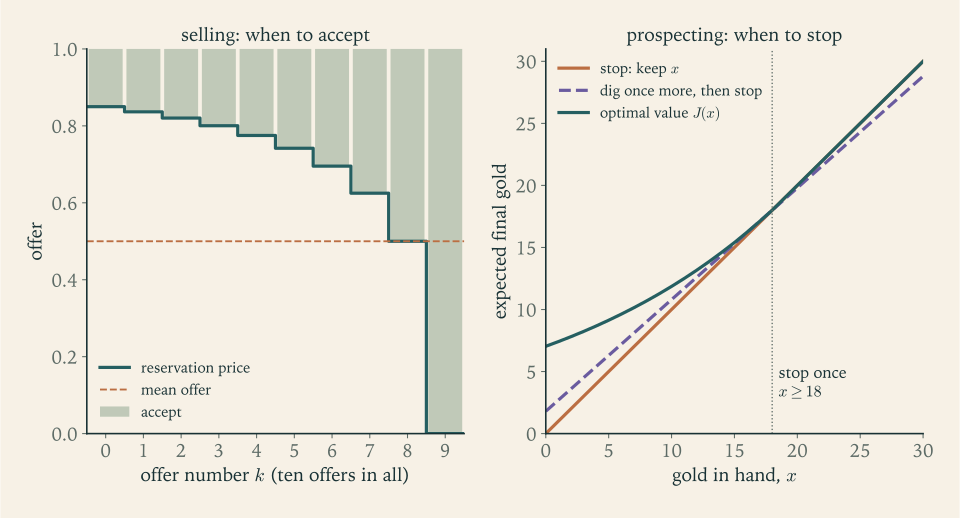
With five offers in all, the seller accepts the first offer only if it is at least \(V_4\approx0.742\) , the second if at least \(0.695\) , the third if at least \(\tfrac58\) , the fourth if at least \(\tfrac12\) , and the fifth whatever it is. The expected sale price is \(V_5\approx0.775\) .
Two simpler rules for comparison. Accepting the first offer yields \(0.5\) . Accepting the first offer above the mean \(\tfrac12\) , and the last if none is, yields \(\tfrac{47}{64}\approx0.734\) . Even the best single fixed threshold, about \(0.67\) , yields only \(0.767\) . The last part of the gain comes from letting the threshold decline, and Section 8.4 returns to why the rule based on the mean falls short.
Common mistake. Raising the threshold as the deadline nears, “to make up for the offers already passed over”. Past offers are gone, and they do not enter the recursion at all. The only thing that changes from one stage to the next is the continuation value \(V_n\) , and it falls as \(n\) falls, because there are fewer chances left. A seller who has rejected three good offers and has two left should be less demanding than at the start, however galling that is.
8.3 No deadline
Remove the deadline and let the offers continue for ever, but let waiting be costly: a reward received \(k\) periods from now is multiplied by \(\alpha^{k}\) , with \(0<\alpha<1\) . Nothing now depends on the stage, so the reservation price should be a single number.
Theorem 8.3 (stationary reservation price). Let the offers be independent with a common distribution on a bounded interval \([0,M]\) , and let rewards be discounted by \(\alpha\in(0,1)\) per period. The equation
has exactly one solution \(a^\star\) . With an offer \(x\) in hand the optimal expected reward is \(\max\{x,a^\star\}\) , and it is optimal to accept the first offer that is at least \(a^\star\) .
Proof. Let \(\phi(a)=\alpha E[\max\{w,a\}]\) . For all \(a,a'\) and every \(w\) , \(\lvert\max\{w,a\}-\max\{w,a'\}\rvert\le\lvert a-a'\rvert\) , so \(\lvert\phi(a)-\phi(a')\rvert\le\alpha\lvert a-a'\rvert\) . As in Theorem 4.5, a contraction of the real line has exactly one fixed point \(a^\star\) , and the iterates \(a_{n+1}=\phi(a_n)\) from \(a_0=0\) converge to it.
By the argument of Theorem 8.2 with discounting, \(a_n\) is the continuation value when at most \(n\) further offers may be considered. The unrestricted continuation value \(a_\infty\) satisfies \(a_n\le a_\infty\le a_n+\alpha^{n}M\) : the lower bound because a seller without a deadline can imitate one with a deadline, the upper because anything received after more than \(n\) periods is worth at most \(\alpha^{n}M\) . Letting \(n\to\infty\) gives \(a_\infty=a^\star\) . So with \(x\) in hand the optimal reward is \(\max\{x,a^\star\}\) .
The threshold rule attains it. Let \(v\) be the expected reward of the rule, before an offer is seen. The next offer is accepted if it is at least \(a^\star\) , and otherwise the seller is in the same position one period later: \(v=E[w;\,w\ge a^\star]+P(w<a^\star)\,\alpha v\) , where \(E[w;\,w\ge a^\star]\) denotes the expectation of \(w\) over the event shown. The fixed-point equation reads \(\tfrac{a^\star}{\alpha}=E[w;\,w\ge a^\star]+P(w<a^\star)\,a^\star\) , so \(v=\tfrac{a^\star}{\alpha}\) solves the linear equation for \(v\) , whose solution is unique. The rule’s continuation value is therefore \(\alpha v=a^\star\) .
Example 8.2: An impatient seller
For offers uniform on \([0,1]\) the equation is \(a=\tfrac{\alpha}{2}(1+a^{2})\) , a quadratic with the root in \([0,1]\)
For \(\alpha=0.9\) , \(a^\star\approx0.627\) ; for \(\alpha=0.99\) , \(a^\star\approx0.868\) ; for \(\alpha=0.5\) , \(a^\star\approx0.268\) . A seller with \(\alpha=0.99\) holds out for roughly the top eighth of offers; a seller who values tomorrow at half of today takes almost anything.
The finite-horizon thresholds with discounting, \(a_{n+1}=\tfrac{0.9}{2}(1+a_n^{2})\) from \(a_0=0\) , are \(0.45\) , \(0.541\) , \(0.582\) , \(0.602,\dots\) , increasing to \(0.627\) . A deadline matters only when it is near.
8.4 Looking one step ahead
Computing a continuation value requires solving the whole problem from the next stage on. There is a much cheaper comparison: stop now, against continue for exactly one stage and then stop. The states at which stopping wins that comparison form the one-step look-ahead set
Since \(J_{k+1}\ge t_{k+1}\) , the true continuation value is at least the one-step value, so \(T_k\subseteq B_k\) : wherever stopping is optimal, it also wins the one-step comparison. The converse is false in general. It is true under one condition.
Theorem 8.4 (one-step look-ahead). Suppose that the sets \(B_k\) are absorbing: for every \(k\) and every \(x\in B_k\) , if the decision maker continues from \(x\) , then \(x_{k+1}\in B_{k+1}\) with probability \(1\) . Take \(B_N\) to be the whole state set. Then \(T_k=B_k\) for every \(k\) : the policy that stops at the first stage \(k\) with \(x_k\in B_k\) is optimal.
Proof. By backward induction we show that \(J_k(x)=t_k(x)\) for \(x\in B_k\) and that continuing is strictly better than stopping for \(x\notin B_k\) . At \(k=N\) stopping is compulsory and \(J_N=t_N\) . Suppose \(J_{k+1}=t_{k+1}\) on \(B_{k+1}\) . If \(x\in B_k\) , then by the absorbing property \(x_{k+1}\in B_{k+1}\) with probability \(1\) , so the continuation value is \(c_k(x)+E[J_{k+1}(x_{k+1})]=c_k(x)+E[t_{k+1}(x_{k+1})]\le t_k(x)\) , by the definition of \(B_k\) . Stopping is optimal and \(J_k(x)=t_k(x)\) . If \(x\notin B_k\) , the continuation value is at least \(c_k(x)+E[t_{k+1}(x_{k+1})]\) , which exceeds \(t_k(x)\) ; so continuing is strictly better.
The absorbing property says that once stopping looks right, it keeps looking right. It holds typically when something accumulates and cannot be undone.
Example 8.3: The prospector
A prospector has dug \(x\) ounces of gold from a shaft. Each further dig brings the roof down with probability \(0.1\) , in which case everything is lost and the venture ends with nothing; otherwise it yields \(1\) , \(2\) , or \(3\) ounces with equal probability. The prospector may walk away at any time with the gold in hand, and can make at most \(N\) digs.
Stopping with \(x\) yields \(x\) . Digging once more and then stopping yields \(0.9\,(x+2)\) in expectation. So
the same set at every stage. From a state in \(B\) a further dig leads either to a larger amount of gold, again in \(B\) , or to the end of the venture, where there is nothing left to decide. The sets are absorbing, and by Theorem 8.4 the optimal policy is: dig until at least \(18\) ounces are in hand, then leave.
At \(x=17\) one more dig is worth \(0.9\cdot19=17.1\) , slightly better than leaving. At \(x=18\) it is worth exactly \(18\) , a tie. The rule does not depend on \(N\) . Solving the recursion numerically for a large number of permitted digs confirms the stopping set and gives \(J(0)\approx7.04\) : starting with nothing, the venture is worth about \(7\) ounces, well under the \(18\) at which the prospector would stop, because most ventures end under a collapsed roof before reaching it.
Example 8.4: Where one step is not enough
Apply the one-step comparison to the asset sale of Example 8.1. Stopping with offer \(x\) yields \(x\) ; continuing one stage and then stopping yields the mean offer \(\tfrac12\) . So \(B=\{x\ge\tfrac12\}\) at every stage with offers still to come: accept any offer above the mean.
This is the second rule of Example 8.1, and it is not optimal: with five offers it yields \(0.734\) against \(0.775\) . The theorem does not apply, because \(B\) is not absorbing. From an offer of \(0.6\) , which is in \(B\) , continuing leads to a fresh offer that falls below \(\tfrac12\) half the time. The one-step comparison assumes the seller would stop at the next stage, when in fact the seller would stop there only if the next offer were good. It ignores the option to continue again, and so it undervalues continuing.
The comparison between the two examples is the content of the theorem. For the prospector, the option to continue again is worthless once \(x\ge18\) , because the situation only becomes less favourable to digging as gold accumulates. For the seller, the option is valuable at every stage but the last.
There is a tidy special case in which no computation is needed at all. If there is no reward for continuing and the stopping reward is a martingale, meaning \(E[t_{k+1}(x_{k+1})\mid x_k=x]=t_k(x)\)
for all \(x\)
and \(k\)
, then the recursion gives \(J_k=t_k\)
by induction: every stopping rule with a bounded horizon earns the same expected reward as stopping at once. No amount of cleverness about timing beats a fair game, a fact about martingales from Stochastic Processes (math.stochastic-processes.martingale-fair-game).
8.5 Choosing the best
The last example has no numbers attached to the candidates at all, only comparisons.
Example 8.5: The best of ten candidates
Ten candidates are interviewed in random order, all orderings being equally likely. After each interview the candidate must be accepted or rejected for good, and the interviewer can only rank the candidates seen so far. The aim is to maximize the probability of choosing the best of the ten.
Two facts about random orderings are needed. The \(k\) -th candidate is the best of the first \(k\) with probability \(\tfrac1k\) , independently of the relative order of the earlier ones; and a candidate who is the best of the first \(k\) is the best of all \(N\) with probability \(\tfrac kN\) .
Accepting a candidate who is not the best so far wins with probability \(0\) , so the only real decisions occur at candidates who are. Let \(V_k\) be the largest achievable probability of success when \(k\) candidates have been rejected. Then \(V_N=0\) and, considering candidate \(k\) ,
The recursion shows \(V_{k-1}\ge V_k\) , so \(V_k\) decreases as \(k\) grows while \(\tfrac kN\) increases. Hence there is a cut-off \(r\) : accept a best-so-far candidate at position \(k\) if and only if \(k\ge r\) .
For \(N=10\) , working backward: \(V_9=\tfrac1{10}\) , \(V_8=\tfrac19\cdot\tfrac{9}{10}+\tfrac89\cdot\tfrac1{10}=\tfrac{17}{90}\) , and so on down to \(V_3=\tfrac{3349}{8400}\approx0.3987\) . At \(k=4\) , \(\tfrac{4}{10}\ge V_4\approx0.3983\) , so a best-so-far fourth candidate is accepted; at \(k=3\) , \(\tfrac{3}{10}\) is less than \(V_3\) , so a best-so-far third candidate is passed over. The optimal rule is to let the first three candidates go and then take the first who is better than all before. It succeeds with probability \(\tfrac{3349}{8400}\approx0.399\) .
For comparison, the success probabilities of cut-off rules that pass over the first \(2\) , \(3\) , and \(4\) candidates are \(0.366\) , \(0.399\) , and \(0.398\) , and choosing at random succeeds with probability \(0.1\) . As \(N\) grows the optimal rule passes over a fraction of the candidates that tends to \(1/e\approx0.368\) , and its success probability tends to the same number: with a hundred candidates, pass over \(37\) and succeed with probability \(0.371\) .
The structure of the answer is the structure of the whole chapter. Early on, the continuation value is high, because much remains to be seen, and stopping is not worth it even at a candidate who looks best. Later the continuation value has fallen below what stopping offers. The threshold is where the two cross.
A stopping problem has a discrete decision. Chapter 9 goes to the opposite extreme: a control that can be adjusted continuously, in continuous time. The Bellman recursion becomes a partial differential equation, and the comparison of stopping against continuing reappears, in a different form, as a control that switches between its extreme values.
Exercises
-
Write the dynamic programming recursion for a stopping problem with stopping rewards \(t_k\) and continuation rewards \(c_k\) , define the stopping set \(T_k\) and the one-step look-ahead set \(B_k\) , and state the inclusion that always holds between them.
Hint
\(J_N=t_N\) and \(J_k(x)=\max\{t_k(x),\ c_k(x)+E[J_{k+1}(x_{k+1})\mid x_k=x]\}\) . \(T_k\) compares stopping with the full continuation value, \(B_k\) with the value of continuing one stage and then stopping. Since \(J_{k+1}\ge t_{k+1}\) , the full continuation value is the larger, so \(T_k\subseteq B_k\) .
-
For offers uniformly distributed on \([0,1]\) and four offers in all, list the reservation price that applies to each of the four offers and compute the expected sale price.
Solution
By Theorem 8.2 the threshold for an offer is \(V_n\) , where \(n\) is the number of offers still to come after it, and for uniform offers \(V_{n+1}=\tfrac12(1+V_n^{2})\) with \(V_0=0\) . So \(V_1=\tfrac12\) , \(V_2=\tfrac12\big(1+\tfrac14\big)=\tfrac58\) , and \(V_3=\tfrac12\big(1+\tfrac{25}{64}\big)=\tfrac{89}{128}\approx0.695\) .
With four offers in all, three remain after the first, two after the second, one after the third, and none after the fourth. The reservation prices are therefore \(\tfrac{89}{128}\) for the first offer, \(\tfrac58\) for the second, \(\tfrac12\) for the third, and \(0\) for the fourth, which must be taken.
The expected sale price is the value with four offers to come and none in hand, \(V_4=\tfrac12\big(1+V_3^{2}\big)=\tfrac{24305}{32768}\approx0.7417\) . Each additional offer is worth less than the one before: the gains are \(0.5\) , \(0.125\) , \(0.070\) , \(0.046\) .
-
Offers take the values \(1\) , \(2\) , \(3\) with probability \(\tfrac13\) each, and there are three offers in all. Compute \(V_1\) , \(V_2\) , \(V_3\) , and describe the optimal policy offer by offer.
Solution
Use \(V_{n+1}=E[\max\{w,V_n\}]\) with \(V_0=0\) and \(w\) equal to \(1\) , \(2\) , \(3\) with probability \(\tfrac13\) each.
\(V_1=E[w]=2\) . \(V_2=\tfrac13\big(\max\{1,2\}+\max\{2,2\}+\max\{3,2\}\big)=\tfrac13(2+2+3)=\tfrac73\) . Since \(\tfrac73\) lies between \(2\) and \(3\) , \(V_3=\tfrac13\big(\tfrac73+\tfrac73+3\big)=\tfrac{23}{9}\approx2.56\) .
Policy. The first offer is accepted if it is at least \(V_2=\tfrac73\) , that is, only if it is \(3\) . The second offer is accepted if it is at least \(V_1=2\) : an offer of \(3\) is accepted, an offer of \(1\) is rejected, and at an offer of \(2\) the seller is indifferent, since waiting for the last offer is worth \(2\) on average. The third offer is accepted whatever it is.
The expected sale price is \(\tfrac{23}{9}\) , against \(2\) for taking the first offer. With a discrete distribution the threshold \(\tfrac73\) is not itself a possible offer; what matters is which offers lie above it.
-
For offers uniform on \([0,1]\) let \(d_n=1-V_n\) . Show that \(d_{n+1}=d_n\big(1-\tfrac12d_n\big)\) , deduce that \(d_n\) decreases to \(0\) , and interpret the limit.
Solution
From \(V_{n+1}=\tfrac12(1+V_n^{2})\) ,
\[ d_{n+1}=1-V_{n+1}=\tfrac12\big(1-V_n^{2}\big)=\tfrac12(1-V_n)(1+V_n)=\tfrac12d_n(2-d_n)=d_n\big(1-\tfrac12d_n\big). \]Start from \(d_0=1\) . If \(0<d_n\le1\) then \(\tfrac12\le1-\tfrac12d_n<1\) , so \(0<d_{n+1}<d_n\) : the sequence is positive and strictly decreasing, hence convergent to some limit \(d\ge0\) . Passing to the limit in the recursion, \(d=d\,(1-\tfrac12d)\) , so \(\tfrac12d^{2}=0\) and \(d=0\) .
So \(V_n\to1\) : with enough offers still to come, the seller can expect a price as close as desired to the largest possible offer, by holding out for it. The convergence is slow, though. Since \(\dfrac1{d_{n+1}}=\dfrac{1}{d_n}\cdot\dfrac{1}{1-\tfrac12d_n}\approx\dfrac1{d_n}+\dfrac12\) , the gap behaves like \(\dfrac2n\) for large \(n\) : a hundred offers leave a gap of about \(0.02\) .
-
For offers uniform on \([0,1]\) with discount factor \(\alpha=0.5\) and no deadline, compute the reservation price from Theorem 8.3, verify that it satisfies the fixed-point equation, and compute the expected discounted reward of the optimal rule before any offer is seen.
Solution
For uniform offers \(a^\star=\dfrac{1-\sqrt{1-\alpha^{2}}}{\alpha}\) . With \(\alpha=\tfrac12\) : \(\sqrt{1-\tfrac14}=\tfrac{\sqrt3}{2}\) , so \(a^\star=2\big(1-\tfrac{\sqrt3}{2}\big)\) , that is, \(a^\star=2-\sqrt3\approx0.268\) .
Check the fixed-point equation \(a=\tfrac{\alpha}{2}(1+a^{2})\) : \((2-\sqrt3)^{2}=7-4\sqrt3\) , so \(\tfrac14\big(1+7-4\sqrt3\big)=2-\sqrt3\) , as required.
By the proof of Theorem 8.3 the expected discounted reward before an offer is seen is \(v=\dfrac{a^\star}{\alpha}=2\,(2-\sqrt3)\approx0.536\) . This is only slightly above the mean offer \(0.5\) : with so heavy a discount, waiting even one period halves the reward, and the seller rejects only the worst quarter or so of offers.
-
Suppose there is no discounting and no deadline, but each rejected offer costs the seller \(c\) . Argue that the reservation price \(a\) satisfies \(c=E[\max\{w-a,0\}]\) , and solve the equation for offers uniform on \([0,1]\) with \(c=0.02\) .
Answer
With offer \(x\) in hand the value is \(\max\{x,a\}\) , where \(a\) is the value of rejecting: \(a=-c+E[\max\{w,a\}]\) . Subtracting \(a\) from both sides gives \(c=E[\max\{w-a,0\}]\) : the reservation price is the level at which the expected gain from one more offer equals its cost. For uniform offers \(E[\max\{w-a,0\}]=\tfrac12(1-a)^{2}\) , so \(a=1-\sqrt{2c}\) , which is \(0.8\) for \(c=0.02\) .
-
In Example 8.3 change the probability of collapse to \(0.2\) . Find the one-step look-ahead set and the optimal rule. Then suppose in addition that each dig costs \(0.5\) ounce in supplies, and find the new threshold.
Solution
With collapse probability \(0.2\) , digging once more and then stopping yields \(0.8\,(x+2)\) . Stopping is at least as good when \(x\ge0.8x+1.6\) , that is, \(x\ge8\) . The set \(\{x\ge8\}\) is absorbing for the same reason as in Example 8.3: a successful dig only increases \(x\) , and a collapse ends the venture. By Theorem 8.4 the optimal rule is to dig until at least \(8\) ounces are in hand. Doubling the risk more than halved the threshold, from \(18\) to \(8\) .
With a cost of \(0.5\) per dig, digging once more and then stopping yields \(0.8\,(x+2)-0.5\) , and stopping is at least as good when \(0.2x\ge1.1\) , that is, \(x\ge5.5\) . Since the gold comes in whole ounces, the rule is to stop once \(x\ge6\) . The set is still absorbing, so the rule is optimal.
In both cases the threshold has the form “expected gain from one more dig, divided by the probability of losing everything”: \(\dfrac{0.8\cdot2}{0.2}=8\) and \(\dfrac{0.8\cdot2-0.5}{0.2}=5.5\) . The prospector stops when the stake at risk has grown to the point where the expected loss from a collapse equals the expected gain from a successful dig.
-
A seller with five uniformly distributed offers adopts the rule “accept the first offer above the average offer”. Compute the expected sale price of this rule, compare it with the optimal one, and identify the hypothesis of Theorem 8.4 that fails for this problem.
Solution
The rule accepts each of the first four offers if it exceeds \(\tfrac12\) , and takes the fifth otherwise. An offer above \(\tfrac12\) has conditional mean \(\tfrac34\) and occurs with probability \(\tfrac12\) . The probability that one of the first four is accepted is \(1-\big(\tfrac12\big)^{4}=\tfrac{15}{16}\) ; otherwise, with probability \(\tfrac1{16}\) , the last offer is taken, with mean \(\tfrac12\) . The expected price is \(\tfrac{15}{16}\cdot\tfrac34+\tfrac1{16}\cdot\tfrac12=\tfrac{47}{64}\approx0.734\) .
The optimal policy yields \(V_5\approx0.775\) , so the rule loses about \(0.04\) , or \(5\) percent.
The rule is the one-step look-ahead rule, since \(\tfrac12\) is what continuing once and then stopping would bring. Theorem 8.4 would make it optimal if the set \(B=\{x\ge\tfrac12\}\) were absorbing. It is not: the state is the current offer, and after a rejection the next offer is a fresh draw that lies below \(\tfrac12\) with probability \(\tfrac12\) . The one-step comparison undervalues continuing because it ignores the seller’s option to reject the next offer too.
-
A student argues that the reservation price should rise as the deadline approaches, “because a seller who has turned down good offers needs a higher price to justify having waited”. Explain, with reference to the recursion of Theorem 8.2, why the argument is wrong and what quantity actually determines the threshold.
Hint
Look at what enters \(V_{n+1}=E[\max\{w,V_n\}]\) : the distribution of future offers and the number of them remaining. The offers already rejected appear nowhere. The threshold is the continuation value, and with fewer offers left there is less to continue for, so it falls. What the seller “needs to justify having waited” is a sunk consideration.
-
For five candidates in the setting of Example 8.5, compute \(V_4,V_3,V_2,V_1,V_0\) , find the optimal cut-off, and state the probability of success.
Solution
With \(N=5\) the recursion is \(V_5=0\) and \(V_{k-1}=\tfrac1k\max\{\tfrac k5,V_k\}+\tfrac{k-1}{k}V_k\) .
\(k=5\) : \(V_4=\tfrac15\cdot1+\tfrac45\cdot0=\tfrac15\) . The last candidate, if best so far, is certainly the best.
\(k=4\) : \(\tfrac45\ge V_4=\tfrac15\) , so accept; \(V_3=\tfrac14\cdot\tfrac45+\tfrac34\cdot\tfrac15=\tfrac{7}{20}\) .
\(k=3\) : \(\tfrac35\ge V_3=\tfrac{7}{20}\) , so accept; \(V_2=\tfrac13\cdot\tfrac35+\tfrac23\cdot\tfrac{7}{20}=\tfrac{13}{30}\) .
\(k=2\) : \(\tfrac25=\tfrac{12}{30}\) is less than \(V_2=\tfrac{13}{30}\) , so pass; \(V_1=V_2=\tfrac{13}{30}\) .
\(k=1\) : \(\tfrac15\) is less than \(V_1\) , so pass; \(V_0=\tfrac{13}{30}\) .
The optimal cut-off is \(r=3\) : let the first two candidates go, then accept the first who is better than all before. The probability of success is \(\tfrac{13}{30}\approx0.433\) , against \(0.2\) for a random choice. At \(k=2\) the decision is close: accepting a best-so-far second candidate would succeed with probability \(0.4\) , and waiting is worth \(0.433\) .
-
In the setting of Example 8.5, show that the rule “pass over the first \(r-1\) candidates and then accept the first who is best so far” succeeds with probability \(\dfrac{r-1}{N}\sum_{k=r}^{N}\dfrac{1}{k-1}\) for \(r\ge2\) , and evaluate it for \(N=10\) and \(r=4\) .
Hint
The rule succeeds if the best candidate is at some position \(k\ge r\) and is reached, which happens when nobody at positions \(r,\dots,k-1\) was accepted. That requires the best of the first \(k-1\) candidates to be among the first \(r-1\) , an event of probability \(\tfrac{r-1}{k-1}\) . The best candidate is at position \(k\) with probability \(\tfrac1N\) . Sum over \(k\) . For \(N=10\) , \(r=4\) : \(\tfrac{3}{10}\big(\tfrac13+\tfrac14+\dots+\tfrac19\big)\approx0.3987\) .
-
Write the asset-selling problem of Section 8.2 as a model in the sense of Definition 1.1, with a state that records whether the asset has been sold, and check that the recursion of Theorem 2.2 for it reduces to the recursion of Theorem 8.2.
Hint
Take the state to be either the current offer or a special value “sold”. From an offer \(x\) the control “accept” earns \(x\) and moves to “sold”; “reject” earns \(0\) and moves to the next offer \(w_{k+1}\) , which is the disturbance. From “sold” there is one control, earning \(0\) and staying. At the last stage only “accept” is admissible. The recursion gives \(J_k(\text{sold})=0\) and \(J_k(x)=\max\{x,\ E[J_{k+1}(w)]\}\) .
-
A stock price is \(4\) now and at each of two steps is multiplied by \(2\) with probability \(\tfrac13\) or by \(\tfrac12\) with probability \(\tfrac23\) . The holder of an option may stop at any time and receive \(\max\{5-S,0\}\) , where \(S\) is the current price, and must stop after two steps. Compute the optimal expected reward and the stopping set, and explain the result using the fact that the price is a martingale and the reward is a convex function of it.
Solution
The prices are \(4\) at step \(0\) ; \(8\) or \(2\) at step \(1\) ; \(16\) , \(4\) , or \(1\) at step \(2\) . The stopping reward is \(r(S)=\max\{5-S,0\}\) .
Step 2. Stopping is compulsory: \(J_2=0\) , \(1\) , \(4\) at prices \(16\) , \(4\) , \(1\) .
Step 1. At price \(8\) : stopping yields \(0\) ; continuing yields \(\tfrac13\cdot0+\tfrac23\cdot1=\tfrac23\) . Continue; \(J_1(8)=\tfrac23\) . At price \(2\) : stopping yields \(3\) ; continuing yields \(\tfrac13\cdot1+\tfrac23\cdot4=3\) . A tie; \(J_1(2)=3\) .
Step 0. At price \(4\) : stopping yields \(1\) ; continuing yields \(\tfrac13\cdot\tfrac23+\tfrac23\cdot3=\tfrac{20}{9}\) . Continue. The optimal expected reward is \(\tfrac{20}{9}\approx2.22\) , and stopping before the end is never strictly better; the only early stopping state is the tie at price \(2\) .
The reason is general. The price is a martingale: \(\tfrac13\cdot2S+\tfrac23\cdot\tfrac12S=S\) . The reward \(r\) is a convex function, and for a convex function the average of its values is at least its value at the average, so \(E[r(S_{k+1})\mid S_k]\ge r(S_k)\) . Continuing one stage and then stopping is therefore at least as good as stopping now, in every state, and by induction waiting until the end is optimal. With discounting, or with a price that tends to drift, this argument fails and early stopping can become optimal.
-
In the problem of Exercise 13, replace the reward by the price itself, so that stopping at price \(S\) yields \(S\) . Show without computing a table that every stopping rule has expected reward \(4\) .
Answer
The price satisfies \(E[S_{k+1}\mid S_k]=\tfrac13\cdot2S_k+\tfrac23\cdot\tfrac12S_k=S_k\) , so the stopping reward is a martingale and there is no reward for continuing. The recursion gives \(J_2=S\) , then \(J_1(S)=\max\{S,S\}=S\) , then \(J_0(4)=4\) , with every choice tied at every state. Every stopping rule has expected reward \(4\) .
-
A machine is bad with probability \(p\) . The inspector may accept it, at an expected cost of \(10p\) , or reject it, at an expected cost of \(3(1-p)\) , or first observe one item at a cost of \(0.5\) and then accept or reject, where an item is defective with probability \(0.6\) from a bad machine and \(0.1\) from a good one. Find the set of beliefs \(p\) for which observing first is the best of the three options.
Solution
Stopping at once costs \(s(p)=\min\{10p,\ 3(1-p)\}\) : accept if \(p\le\tfrac{3}{13}\) , reject otherwise.
Observing costs \(0.5\) and then the better of the two terminal actions at the posterior belief. As in Example 7.2, the probability of an observation times the terminal cost at its posterior is linear in \(p\) : after a defective item the two terminal costs contribute \(10\cdot0.6\,p=6p\) for accepting and \(3\cdot0.1\,(1-p)=0.3\,(1-p)\) for rejecting; after a sound item, \(4p\) and \(2.7\,(1-p)\) .
For \(p\) between \(\tfrac1{21}\) and about \(0.40\) the best continuation is to reject after a defective item and accept after a sound one, and observing costs
\[ 0.5+0.3\,(1-p)+4p=0.8+3.7\,p . \]Compare with stopping. Against accepting: \(0.8+3.7p<10p\) when \(p>\tfrac{0.8}{6.3}=\tfrac{8}{63}\approx0.127\) . Against rejecting: \(0.8+3.7p<3-3p\) when \(p<\tfrac{2.2}{6.7}=\tfrac{22}{67}\approx0.328\) . Both bounds lie inside the range where the contingent continuation is the best one, and outside that range observing cannot pay, since the observation would not change the action.
So observing first is best exactly when \(\tfrac{8}{63}<p<\tfrac{22}{67}\) . For smaller \(p\) accept at once; for larger \(p\) reject at once. The policy has two thresholds, with a region of doubt between them in which information is bought. This is the pattern of sequential testing: a stopping problem on the belief space of Chapter 7.
-
Prove the version of Theorem 8.4 for costs: if stopping costs \(t_k(x)\) , continuing costs \(c_k(x)\) , the objective is to minimize, and the sets \(B_k=\{x:\ t_k(x)\le c_k(x)+E[t_{k+1}(x_{k+1})\mid x_k=x]\}\) are absorbing, then stopping at the first entry into \(B_k\) is optimal.
Hint
Repeat the proof of Theorem 8.4 with minima and reversed inequalities: the optimal cost satisfies \(J_{k+1}\le t_{k+1}\) , so the true continuation cost is at most the one-step continuation cost, and outside \(B_k\) continuing is strictly cheaper than stopping; inside \(B_k\) the absorbing property gives \(J_{k+1}=t_{k+1}\) at the next state, so the two continuation costs coincide.
-
Suppose the seller of Section 8.2 can recall past offers, so that stopping yields the best offer seen so far, and that each further offer costs \(c\) to obtain, with no discounting. With the best offer so far as the state, find the one-step look-ahead set, show that it is absorbing, and conclude that the optimal rule is a fixed threshold. Compare the threshold with the answer to Exercise 6.
Solution
Let \(m\) be the best offer so far. Stopping yields \(m\) . Paying \(c\) for one more offer and then stopping yields \(-c+E[\max\{w,m\}]\) . Stopping wins the one-step comparison when \(m\ge-c+E[\max\{w,m\}]\) , that is, when
\[ E\big[\max\{w-m,\,0\}\big]\le c . \]The left side is the expected improvement from one more offer. It is a nonincreasing function of \(m\) , so the one-step look-ahead set is \(B=\{m\ge a\}\) , where \(a\) is the smallest level at which the expected improvement is at most \(c\) .
The set is absorbing: the best offer so far can only increase, so once \(m\ge a\) it stays there. By Theorem 8.4, in its finite-horizon form for any number of permitted offers, the optimal rule is to stop at the first time the best offer so far is at least \(a\) . That time is the first time a single offer is at least \(a\) , so the right to recall earlier offers is never used.
For uniform offers \(E[\max\{w-m,0\}]=\tfrac12(1-m)^{2}\) , and \(a=1-\sqrt{2c}\) , which is \(0.8\) for \(c=0.02\) : the same threshold as in Exercise 6, where recall was not allowed. With a stationary threshold an offer once rejected would be rejected again, so recall has no value.
-
For three uniformly distributed offers, write the optimal value \(\max\{x,V_2\}\) with the first offer \(x\) in hand as an explicit function of \(x\) , integrate it over \(x\) to recover \(V_3\) , and sketch the function, marking the threshold.
Answer
With the first of three offers in hand the value is \(J(x)=\tfrac58\) for \(x\le\tfrac58\) and \(J(x)=x\) for \(x\ge\tfrac58\) : flat, then rising along the diagonal, with a kink at the threshold \(\tfrac58\) . Integrating, \(\int_0^1J(x)\,dx=\tfrac58\cdot\tfrac58+\tfrac12\big(1-\tfrac{25}{64}\big)=\tfrac{25}{64}+\tfrac{39}{128}=\tfrac{89}{128}=V_3\) .