A machine is either in good condition or in bad condition, and nobody can see which. What can be seen is its output: each item it makes is either sound or defective, a bad machine makes many more defectives than a good one, and a good machine makes some too. After each item the operator must decide whether to keep producing or to stop and repair.
The methods of the earlier chapters do not apply as they stand. A policy was a function of the state, and here the state is hidden. The observation of the moment is not a state either: one defective item means little, three in a row mean a great deal, so the past matters. The full record of observations is a state, by the test of Chapter 1, but it grows without bound.
The resolution is one of the most useful ideas in the subject. What the operator needs from the past is the conditional probability, given everything seen so far, that the machine is bad. That number can be updated from one stage to the next by Bayes’ rule, and it has the state property. Replacing the hidden state by this probability, the belief, turns a problem with imperfect information into a problem with perfect information on a larger state space, and everything from Chapters 2 to 6 applies to it.
7.1 A model in which the state is hidden
Definition 7.1 (partially observed model). A partially observed Markov decision process consists of a finite set \(S\) of hidden states with transition probabilities \(p_{ij}(u)\) ; a finite set of controls \(U\) , the same in every state; a finite set \(Z\) of observations with probabilities
stage costs \(g(i,u)\) and a terminal cost \(g_N(i)\) ; and an initial distribution \(b_0\) of \(x_0\) . Given \(x_k\) and \(u_k\) , the next state \(x_{k+1}\) is independent of all earlier states, controls, and observations, and given \(x_{k+1}\) and \(u_k\) , the observation \(z_{k+1}\) is independent of everything else up to that time. At stage \(k\) the controller knows the information vector
and a policy is a sequence of functions \(u_k=\mu_k(I_k)\) .
The controls are the same in every state because the controller, not knowing the state, cannot be asked to respect a constraint that depends on it. The cost \(g(x_k,u_k)\) is incurred but not seen; if it were seen it would be an observation.
The information vector has the state property for a perfectly observed problem: it is known, it updates by appending \((u_k,z_{k+1})\) , and the conditional distribution of the next observation given \(I_k\) and \(u_k\) is determined by the model. So the theory of Chapter 2 applies with \(I_k\) as the state. The difficulty is purely one of size: with two possible observations and two controls there are \(4^{k}\) information vectors at stage \(k\) .
7.2 The belief and its recursion
Definition 7.2 (belief). The belief at stage \(k\) is the conditional distribution of the hidden state given the information vector: \(b_k(i)=P(x_k=i\mid I_k)\) for \(i\in S\) .
A belief is a probability vector with one component per hidden state. With two hidden states it is a single number.
Theorem 7.3 (the belief is a state). In the model of Definition 7.1, for every policy:
which is written \(b_{k+1}=\Phi(b_k,u_k,z_{k+1})\) . Moreover the conditional probability of the next observation and the conditional expected stage cost depend on \(I_k\) only through \(b_k\) :
Proof. Fix \(I_k\) ; the control \(u_k=\mu_k(I_k)\) is then determined, so conditioning on \(I_k\) and conditioning on \((I_k,u_k)\) are the same. By the two independence assumptions of Definition 7.1,
Summing over \(j\) gives the formula for \(\sigma\) . Since \(I_{k+1}\) consists of \(I_k\) , \(u_k\) , and \(z_{k+1}\) , Bayes’ rule gives
which is the stated recursion. The cost formula is the definition of conditional expectation.
The recursion is Bayes’ rule from Probability Theory (math.probability-theory.bayes-rule), applied once per stage. For a chain with no controls it is the filtering recursion for hidden Markov models studied in Stochastic Processes (math.stochastic-processes.hidden-markov-filtering); the only addition here is that the transition and observation probabilities are those of the control actually used.
It is best remembered as two steps. Predict: push the belief through the transition, \(\bar b(j)=\sum_ib_k(i)\,p_{ij}(u_k)\) ; this is where the system might be now, before looking. Correct: multiply each component by the likelihood \(r(z\mid j,u_k)\) of what was seen, and renormalize. The denominator is \(\sigma(z\mid b_k,u_k)\) , the probability that the model assigned to the observation before it arrived.
Example 7.1: Tracking a machine nobody can see
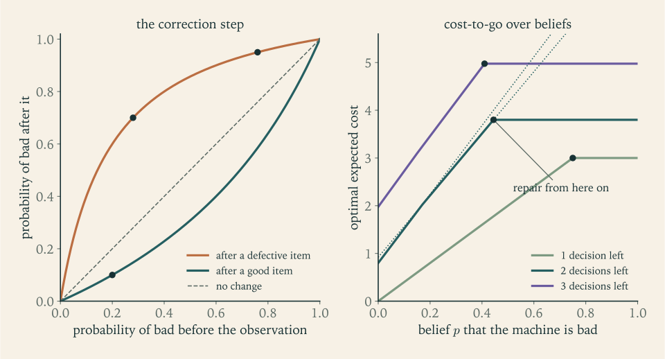
The machine is good or bad. A good machine turns bad with probability \(0.2\) between one item and the next; a bad machine stays bad until repaired. Each item is defective with probability \(0.1\) if the machine was good when it was made and \(0.6\) if it was bad. The belief is \(p_k\) , the probability that the machine is bad.
Predict, when the machine has been left running: \(\bar p=p_k+0.2\,(1-p_k)\) . Correct, on seeing the item:
Start just after a repair, so that \(\bar p=0.2\) for the first item, and suppose the items come out sound, defective, defective.
First item, sound: \(p_1=\dfrac{0.08}{0.08+0.72}=0.1\) . The sound item halves the suspicion.
Second item: predict \(\bar p=0.1+0.2\cdot0.9=0.28\) ; it is defective, so \(p_2=\dfrac{0.168}{0.168+0.072}=0.7\) .
Third item: predict \(\bar p=0.7+0.2\cdot0.3=0.76\) ; defective again, so \(p_3=\dfrac{0.456}{0.456+0.024}=0.95\) .
One defective item took the belief from \(0.28\) to \(0.7\) ; the second took it to \(0.95\) . The probabilities the model assigned to the three observations were \(0.8\) , \(0.24\) , and \(0.48\) : the second defect was twice as expected as the first.
Common mistake. Omitting the prediction step. Applying the correction for a defective item directly to \(p_1=0.1\) gives \(\dfrac{0.06}{0.06+0.09}=0.4\) in place of the correct \(0.7\) . The belief \(p_k\) describes the machine when item \(k\) was made; the next item is made by the machine one transition later, and the likelihoods must be applied to the predicted belief. The error is invisible when the hidden state cannot change, which is why it survives in code that was first tested on a static problem.
A warning about the denominator. If an observation arrives to which the model assigns probability zero, \(\sigma(z\mid b_k,u_k)=0\) , the recursion divides by zero. That is the model saying that what happened is impossible according to it. The honest response is to treat the model as refuted and widen it, for example by making every likelihood slightly positive.
7.3 Dynamic programming over beliefs
Theorem 7.3 says that the belief passes the test of Definition 1.4: it is known to the controller, it determines the expected stage cost and the distribution of the next observation, and with the control and the next observation it determines its own successor. The partially observed problem is therefore equivalent to a perfectly observed one whose state is \(b_k\) , whose disturbance is \(z_{k+1}\) with distribution \(\sigma(\cdot\mid b_k,u_k)\) , and whose system function is \(\Phi\) . By Theorem 2.2 and Theorem 6.2, applied with the information vector as the state, an optimal policy can be taken to be a function of the belief, and
The state space of this problem is the set of all probability vectors on \(S\) , a continuum, so no table can hold \(J_k\) . What saves the computation, for short horizons, is a structural fact.
Theorem 7.4 (cost-to-go functions are piecewise linear and concave). For each \(k\) there is a finite set \(\mathcal A_k\) of vectors in \(\mathbb R^{S}\) such that
In particular \(J_k\) is a concave function of \(b\) .
Proof. By backward induction. \(J_N\) is linear, with \(\mathcal A_N=\{g_N\}\) . Suppose the claim holds at \(k+1\) . For fixed \(u\) and \(z\) ,
because the denominator of \(\Phi\) is \(\sigma(z\mid b,u)\) and cancels. Each expression under the minimum is linear in \(b\) . A sum over \(z\) of minima of linear functions is the minimum, over all ways of choosing one \(a\) for each \(z\) , of the corresponding sums, each of which is linear; adding the linear function \(\sum_ib(i)g(i,u)\) and taking the minimum over the finitely many \(u\) again gives a minimum of finitely many linear functions. A minimum of linear functions is concave.
Each vector in \(\mathcal A_k\) has a meaning: it is the cost vector, indexed by the true hidden state, of one particular plan that says what to do now and what to do after each possible sequence of future observations. \(J_k(b)\) is the cost of the plan that is best when the hidden state is weighted by \(b\) . The number of plans can grow very fast with the horizon, as fast as \(\lvert U\rvert\,\lvert\mathcal A_{k+1}\rvert^{\lvert Z\rvert}\) per stage before dominated plans are discarded, and that is the form the curse of dimensionality takes here.
Example 7.2: The last two decisions
Continue Example 7.1 with costs. Running the machine costs \(4\) for a stage in which it is bad and nothing when it is good. A repair costs \(3\) and makes the machine good at once; it may then turn bad before the next item, with the usual probability \(0.2\) . There is no terminal cost. In terms of the belief \(p\) , running has expected stage cost \(4p\) and leads to the predicted belief \(\bar p=0.2+0.8p\) ; repairing costs \(3\) and leads to \(\bar p=0.2\) .
One decision left. \(J_{N-1}(p)=\min\{4p,\ 3\}\) : run if \(p\le\tfrac34\) , repair otherwise. Two linear pieces, \(\mathcal A_{N-1}=\{(0,4),\ (3,3)\}\) in the coordinates (good, bad).
Two decisions left. If the machine is run now, the next belief is \(p'\) with \(\sigma(z)\,J_{N-1}(p')=\min\{4\,r(z\mid\text{bad})\,\bar p,\ 3\,\sigma(z)\}\) :
After a sound item running is better whenever \(\bar p\le\tfrac{27}{31}\) . After a defective item running is better only if \(\bar p\le\tfrac13\) , that is, \(p\le\tfrac16\) . So there are two plans that start by running:
“run, then run whatever happens” costs \(4p+4\bar p=0.8+7.2\,p\) ;
“run, then repair if the item is defective” costs \(4p+(0.3+1.5\,\bar p)+1.6\,\bar p=0.92+6.48\,p\) .
A third plan, to run and then repair whatever happens, costs \(4p+3\) and is never the cheapest. If the machine is repaired now, \(\bar p=0.2\) , which is below \(\tfrac13\) , so the continuation is to run, and the cost is \(3+4\cdot0.2=3.8\) . Therefore
The first two lines cross at \(p=\tfrac16\) and the second meets the third at \(p=\tfrac49\) . The optimal policy with two decisions left: for \(p\le\tfrac16\) , run now and next time regardless; for \(\tfrac16\le p\le\tfrac49\) , run now and repair next time if the item is defective; for \(p\ge\tfrac49\) , repair now.
The repair threshold has dropped from \(\tfrac34\) to \(\tfrac49\) . With one more stage ahead, a bad machine left running does damage for longer, so less evidence is needed to justify the repair. With three decisions left the threshold is \(\tfrac{1851}{4516}\approx0.410\) , and with four it is about \(0.399\) .
Common mistake. Acting as if the most likely state were the true state. With one decision left and \(p=0.6\) , the machine is more likely bad than good, and for a machine known to be bad the repair, at \(3\) , is cheaper than running, at \(4\) . But at \(p=0.6\) running has expected cost \(2.4\) and repairing costs \(3\) : running is better. The most likely state discards the \(40\) percent chance that the repair is wasted. The error also runs the other way: with two decisions left and \(p=0.47\) the machine is more likely good, yet the optimal action is to repair. Decisions under partial observation depend on the whole belief and on the costs, and a threshold at one half is correct only by accident.
7.4 What an observation is worth
Concavity of \(J_k\) has a consequence that connects this chapter with Section 6.3.
Proposition 7.5 (observations cannot hurt). Let \(J\) be a concave function on beliefs. For every belief \(b\) and control \(u\) , with predicted belief \(\bar b(j)=\sum_ib(i)p_{ij}(u)\) ,
Proof. The corrected beliefs average back to the predicted belief: \(\sum_z\sigma(z\mid b,u)\,\Phi(b,u,z)(j)=\sum_zr(z\mid j,u)\,\bar b(j)=\bar b(j)\) , since the likelihoods of the possible observations sum to \(1\) . The left side of the claim is therefore a weighted average of values of \(J\) at points whose weighted average is \(\bar b\) , and for a concave function such an average is at most the value at the average point.
The right side is the expected future cost if no observation were made and the controller had to continue with the predicted belief; the left side is the expected future cost with the observation. Information lowers expected cost, by an amount that is zero exactly where \(J\) is linear between the possible posterior beliefs, that is, where the observation would not change the plan.
Example 7.3: Three sensors compared
Take three decisions and an initial belief \(p=0.2\) , and compare three machines that differ only in what the operator sees.
No observation. The belief evolves deterministically: \(\bar p=0.2+0.8p\) after running, \(0.2\) after a repair. Dynamic programming on this deterministic problem gives an optimal cost of \(\tfrac{524}{125}=4.192\) .
The noisy item signal of Example 7.1. The recursion of Example 7.2, carried one stage further, gives \(\tfrac{10811}{3125}\approx3.460\) .
A perfect sensor, which reveals the machine’s condition after each transition. The optimal cost is \(\tfrac{62}{25}=2.48\) .
The noisy signal is worth \(4.192-3.460=0.732\) , and a perfect sensor would be worth a further \(0.980\) . These are the amounts that it would be rational to pay for each over three stages.
7.5 Gaussian beliefs
A belief is in general a whole distribution. In one important case it reduces to two numbers. Let the hidden state be a real number following \(x_{k+1}=x_k+w_k\) , observed through \(z_k=x_k+v_k\) , with independent Gaussian noises \(w_k\) of variance \(q\) and \(v_k\) of variance \(\rho\) , and a Gaussian prior. Then every belief is Gaussian, with a mean \(m_k\) and a variance \(P_k\) , and the two steps of the filter are:
This is the scalar Kalman filter. The correction moves the mean toward the observation by the fraction \(\kappa\) , which is large when the prediction is uncertain compared with the sensor. The variance recursion does not involve the observations at all: how uncertain the controller will be at each stage is known in advance.
Example 7.4: A scalar Kalman filter
Let \(q=1\) , \(\rho=2\) , and a prior with mean \(0\) and variance \(4\) . First observation \(z_1=3\) : predict \(\bar P=5\) ; gain \(\kappa=\tfrac57\) ; mean \(m_1=\tfrac57\cdot3=\tfrac{15}{7}\approx2.14\) ; variance \(P_1=\tfrac27\cdot5=\tfrac{10}{7}\) .
Second observation \(z_2=1\) : predict \(\bar P=\tfrac{17}{7}\) ; gain \(\kappa=\tfrac{17}{31}\) ; mean \(m_2=\tfrac{15}{7}+\tfrac{17}{31}\big(1-\tfrac{15}{7}\big)=\tfrac{47}{31}\approx1.52\) ; variance \(P_2=\tfrac{34}{31}\approx1.10\) .
The variances \(4\) , \(\tfrac{10}{7}\) , \(\tfrac{34}{31}\) , \(\tfrac{130}{127},\dots\) decrease to the solution of \(P=\dfrac{(P+q)\,\rho}{P+q+\rho}\) , that is, \(P^{2}+P-2=0\) , which is \(P=1\) , with limiting gain \(\kappa=\tfrac12\) . In the long run the new observation and the prediction built from all the earlier ones are given equal weight.
When such a state is to be controlled, with linear dynamics and quadratic cost, a remarkable simplification occurs, which we state without proof: the optimal control is \(u_k=-L_km_k\) , where \(L_k\) are the gains of Theorem 3.5 and \(m_k\) is the mean of the belief. Estimation and control separate: the filter is designed without reference to the cost, the gains without reference to the noise. Certainty equivalence, in the sense of Section 6.4, holds with the conditional mean in place of the unseen state. As there, the property is special to the linear-quadratic-Gaussian family, and the machine of Example 7.2 shows how badly its analogue fails elsewhere.
The belief idea returns in Chapter 8 in a problem where the only decision is when to stop observing, and in Chapter 10, where the size of belief spaces is one of the reasons exact dynamic programming must be given up.
Exercises
-
Define the information vector and the belief of a partially observed model, and write the belief recursion as a prediction step followed by a correction step, saying which model probabilities each step uses.
Hint
\(I_k\) lists the observations \(z_1,\dots,z_k\) and the controls \(u_0,\dots,u_{k-1}\) ; \(b_k(i)=P(x_k=i\mid I_k)\) . Prediction uses the transition probabilities of the control applied: \(\bar b(j)=\sum_ib_k(i)p_{ij}(u_k)\) . Correction uses the observation likelihoods: multiply \(\bar b(j)\) by \(r(z_{k+1}\mid j,u_k)\) and divide by the sum over \(j\) .
-
In the machine of Example 7.1 let the predicted belief be \(\bar p=0.5\) . Compute the belief after a defective item and after a sound item, and the probability of each observation.
Answer
Defective: probability \(0.6\cdot0.5+0.1\cdot0.5=0.35\) , belief \(\tfrac{0.30}{0.35}=\tfrac67\approx0.857\) . Sound: probability \(0.65\) , belief \(\tfrac{0.20}{0.65}=\tfrac{4}{13}\approx0.308\) .
-
For the machine of Example 7.1, start just after a repair and suppose the first item is defective and the second is sound, the machine running throughout. Compute \(p_1\) and \(p_2\) .
Solution
Just after a repair the machine is good, and it may turn bad before the first item with probability \(0.2\) , so the predicted belief for the first item is \(\bar p=0.2\) .
First item, defective: \(p_1=\dfrac{0.6\cdot0.2}{0.6\cdot0.2+0.1\cdot0.8}\) , that is, \(p_1=\dfrac{0.12}{0.12+0.08}=0.6\) .
Predict for the second item, the machine having been left running: \(\bar p=0.6+0.2\cdot0.4=0.68\) .
Second item, sound: the likelihoods are \(0.4\) for a bad machine and \(0.9\) for a good one, so
\[ p_2=\frac{0.4\cdot0.68}{0.4\cdot0.68+0.9\cdot0.32}=\frac{0.272}{0.560}=\tfrac{17}{35}\approx0.486 . \]A defective item followed by a sound one leaves the operator nearly undecided. Compare Example 7.1, where the same two observations in the opposite order led to \(p_2=0.7\) : the order matters here because the machine can deteriorate between items, and a defect seen later is evidence about a machine that has had longer to go bad and that will stay bad.
-
Suppose the machine’s condition cannot change, so that the drift probability is \(0\) in place of \(0.2\) . Show that the odds \(p/(1-p)\) are multiplied by \(6\) for each defective item and by \(\tfrac49\) for each sound one, and conclude that the belief after any sequence of items depends only on how many of each kind were seen.
Solution
With no drift the prediction step does nothing, \(\bar p=p_k\) . For a defective item the correction gives \(p_{k+1}=\dfrac{0.6\,p_k}{0.6\,p_k+0.1\,(1-p_k)}\) and \(1-p_{k+1}=\dfrac{0.1\,(1-p_k)}{0.6\,p_k+0.1\,(1-p_k)}\) . Dividing, the common denominator cancels:
\[ \frac{p_{k+1}}{1-p_{k+1}}=\frac{0.6}{0.1}\cdot\frac{p_k}{1-p_k}=6\cdot\frac{p_k}{1-p_k}. \]For a sound item the same computation with likelihoods \(0.4\) and \(0.9\) gives the factor \(\tfrac{0.4}{0.9}=\tfrac49\) .
After \(d\) defective and \(s\) sound items, in any order, the odds are therefore \(6^{d}\big(\tfrac49\big)^{s}\) times the initial odds, because multiplication is commutative. The belief is a function of the odds, so it depends on the observations only through the counts \(d\) and \(s\) . For a static hidden state the pair of counts is a sufficient statistic; with drift, as Exercise 3 shows, it is not, and the belief itself must be carried.
-
Prove that the corrected beliefs average to the predicted belief, \(\sum_z\sigma(z\mid b,u)\,\Phi(b,u,z)=\bar b\) , and verify the identity numerically for the second item of Example 7.1.
Solution
By the correction formula, \(\sigma(z\mid b,u)\,\Phi(b,u,z)(j)=r(z\mid j,u)\,\bar b(j)\) , the numerator of the recursion, since the denominator is \(\sigma(z\mid b,u)\) . Summing over \(z\) ,
\[ \sum_z\sigma(z\mid b,u)\,\Phi(b,u,z)(j)=\bar b(j)\sum_zr(z\mid j,u)=\bar b(j), \]because for each hidden state \(j\) the likelihoods of the possible observations form a probability distribution and sum to \(1\) . This is the law of total probability: averaging the posterior over what might be observed returns the prior.
For the second item of Example 7.1, \(\bar p=0.28\) . A defective item has probability \(0.24\) and gives belief \(0.7\) . A sound item has probability \(0.76\) and gives belief \(\dfrac{0.4\cdot0.28}{0.76}=\tfrac{14}{95}\approx0.147\) . The average is \(0.24\cdot0.7+0.76\cdot\tfrac{14}{95}=0.168+0.112=0.28\) , as claimed.
-
In Example 7.2 change the repair cost from \(3\) to \(2\) . Find \(J_{N-1}\) and the repair threshold with one decision left, and explain the direction in which the threshold moved.
Answer
\(J_{N-1}(p)=\min\{4p,\ 2\}\) , with threshold \(p=\tfrac12\) : repair when \(p\) exceeds \(\tfrac12\) . The threshold fell from \(\tfrac34\) because a cheaper repair is worth undertaking on weaker evidence. Only at this particular cost ratio does the rule coincide with “act on the more likely state”.
-
For Example 7.2 with two decisions left and belief \(p=0.3\) , state the optimal plan in words, compute its expected cost from the formula for \(J_{N-2}\) , and compute what the other two plans would cost.
Solution
With two decisions left, \(J_{N-2}(p)=\min\{0.8+7.2\,p,\ 0.92+6.48\,p,\ 3.8\}\) , and \(p=0.3\) lies between the breakpoints \(\tfrac16\) and \(\tfrac49\) , so the middle line is the smallest.
Optimal plan. Run the machine now. Look at the next item: if it is defective, repair before the last stage; if it is sound, run again. Its expected cost is \(0.92+6.48\cdot0.3=2.864\) .
The other plans. “Run now and run again whatever happens” costs \(0.8+7.2\cdot0.3=2.96\) . “Repair now, then run” costs \(3.8\) .
To see the plan at work: after running, the predicted belief is \(\bar p=0.2+0.8\cdot0.3=0.44\) . A defective item, which has probability \(0.6\cdot0.44+0.1\cdot0.56=0.32\) , raises the belief to \(\tfrac{0.264}{0.32}=0.825\) , above the last-stage threshold of \(\tfrac34\) , so repair. A sound item lowers it to \(\tfrac{0.176}{0.68}\approx0.259\) , below the threshold, so run. The contingent plan is worth \(0.096\) more than the plan that ignores the observation; that difference is the value of the observation at this belief.
-
A technician reasons: “With belief \(0.6\) the machine is probably bad, and for a bad machine repair is cheaper than running, so repair.” With one decision left in Example 7.2, compute the expected cost of each action at \(p=0.6\) and identify the step of the reasoning that is invalid.
Solution
Running costs \(4\) in a stage in which the machine is bad and nothing otherwise, so at belief \(p=0.6\) its expected cost is \(4\cdot0.6=2.4\) . Repairing costs \(3\) whatever the machine’s condition. With one decision left there is no future to consider, so the comparison is \(2.4\) against \(3\) : running is better by \(0.6\) .
The invalid step is “for a bad machine repair is cheaper than running, so repair”. That comparison, \(3\) against \(4\) , is correct for a machine known to be bad. The technician’s machine is bad with probability \(0.6\) and good with probability \(0.4\) , and in the second case the repair is pure waste. Replacing the belief by its most likely value discards exactly the information about how likely the alternative is. The correct rule compares expected costs under the whole belief, which gives the threshold \(\tfrac34\) : the repair is justified only when the machine is at least three times as likely to be bad as good.
-
A programmer updates the belief of Example 7.1 by applying the correction formula directly to the previous belief. Starting from \(p_1=0.1\) and observing a defective item, compute the programmer’s answer and the correct one, and describe a test case on which the two procedures agree.
Answer
Without the prediction step: \(\dfrac{0.6\cdot0.1}{0.6\cdot0.1+0.1\cdot0.9}=\dfrac{0.06}{0.15}=0.4\) . Correctly: predict \(\bar p=0.28\) , then correct to \(0.7\) . The two procedures agree whenever the hidden state cannot change, that is, when the drift probability is zero; a test on a static machine would not expose the error.
-
Suppose a good machine never produces a defective item, so that the probability \(0.1\) becomes \(0\) . What is the belief after one defective item? What happens to the recursion if the model also says that a bad machine always produces defectives and a sound item is then observed from a machine believed bad with certainty?
Answer
With likelihood \(0\) under “good”, a defective item gives belief \(\dfrac{0.6\,\bar p}{0.6\,\bar p+0}=1\) : one defect is conclusive. If in addition a bad machine always produces defectives, then at belief \(1\) a sound item has probability \(\sigma=0\) under the model, and the correction is \(\tfrac00\) . The observation contradicts the model, and the recursion has no answer to give.
-
For the machine of Example 7.2 with two decisions left and initial belief \(p=0.2\) , compute the optimal cost when the operator sees nothing, when the operator sees the item signal, and when the operator sees the machine’s condition after each transition, and state the value of each kind of observation.
Solution
All three cases share the first stage. At \(p=0.2\) repairing now costs at least \(3\) , more than the alternatives below, so the machine is run, at expected cost \(4\cdot0.2=0.8\) , and the predicted belief is \(\bar p=0.2+0.8\cdot0.2=0.36\) .
No observation. The last decision is taken at belief \(0.36\) : \(\min\{4\cdot0.36,\ 3\}=1.44\) . Total \(2.24\) .
Item signal. From Example 7.2, \(J_{N-2}(0.2)=0.92+6.48\cdot0.2=2.216\) . The plan is to repair at the last stage only after a defective item.
Perfect sensor. The condition is revealed: bad with probability \(0.36\) , in which case the last stage costs \(\min\{4,3\}=3\) ; good otherwise, at cost \(0\) . Total \(0.8+0.36\cdot3=1.88\) .
The item signal is worth \(2.24-2.216=0.024\) and a perfect sensor a further \(2.216-1.88=0.336\) . The noisy signal is worth little here because only one decision remains after it and the belief \(0.36\) is far from the last-stage threshold: only a defective item changes the decision, and then only barely, from a cost of \(0.6\,\bar p\cdot4\) to \(3\,\sigma\) . With three decisions, in Example 7.3, the same signal was worth \(0.732\) .
-
Let \(J(b)=\min_{a\in\mathcal A}\sum_ia(i)b(i)\) for a finite set \(\mathcal A\) . Prove directly from this formula that for beliefs \(b^{1},\dots,b^{m}\) and weights \(\lambda_1,\dots,\lambda_m\ge0\) summing to \(1\) , \(\sum_l\lambda_lJ(b^{l})\le J\big(\sum_l\lambda_lb^{l}\big)\) .
Solution
Let \(\bar b=\sum_l\lambda_lb^{l}\) , and let \(a^\star\in\mathcal A\) attain the minimum defining \(J(\bar b)\) , so that \(J(\bar b)=\sum_ia^\star(i)\bar b(i)\) . A linear function of \(b\) commutes with weighted averages:
\[ J(\bar b)=\sum_ia^\star(i)\sum_l\lambda_lb^{l}(i)=\sum_l\lambda_l\sum_ia^\star(i)\,b^{l}(i). \]For each \(l\) , the inner sum is the value at \(b^{l}\) of one of the linear functions over which \(J(b^{l})\) is the minimum, so it is at least \(J(b^{l})\) . Since the weights \(\lambda_l\) are nonnegative,
\[ J(\bar b)\ \ge\ \sum_l\lambda_lJ(b^{l}). \]The plan \(a^\star\) that is best for the averaged belief is available at each \(b^{l}\) too, but at each \(b^{l}\) a different plan may be better. That is the content of Proposition 7.5: knowing which \(b^{l}\) has occurred allows the plan to be tailored to it.
-
A scalar state drifts with variance \(q=3\) per stage and is observed with noise variance \(\rho=6\) , starting from a known value so that \(P_0=0\) . Compute the gain and the variance after each of the first two observations, and find the limiting variance and gain.
Solution
With \(P_0=0\) , \(q=3\) , \(\rho=6\) . First observation: predict \(\bar P=0+3=3\) ; gain \(\kappa=\dfrac{3}{3+6}=\tfrac13\) ; variance \(P_1=\tfrac23\cdot3=2\) . Second observation: predict \(\bar P=2+3=5\) ; gain \(\kappa=\dfrac{5}{11}\) ; variance \(P_2=\tfrac{6}{11}\cdot5=\tfrac{30}{11}\approx2.73\) .
The limit satisfies \(P=\dfrac{(P+q)\rho}{P+q+\rho}=\dfrac{6\,(P+3)}{P+9}\) , that is, \(P^{2}+9P=6P+18\) , or \(P^{2}+3P-18=0\) , whose positive root is \(P=3\) . The limiting gain is \(\dfrac{3+3}{3+3+6}=\tfrac12\) .
Starting from perfect knowledge, the variance rises, \(0\) , \(2\) , \(2.73\) , toward \(3\) : each stage the drift adds \(3\) and the observation removes a fraction of what is there. In Example 7.4 the variance fell toward its limit from a vague prior. The limit does not depend on the prior, which is why a long-running filter can be operated with the constant gain.
-
Derive the correction step of the scalar Kalman filter: if \(x\) has a Gaussian density with mean \(\bar m\) and variance \(\bar P\) , and \(z=x+v\) with \(v\) Gaussian of variance \(\rho\) independent of \(x\) , show that the conditional density of \(x\) given \(z\) is Gaussian with the mean and variance stated in Section 7.5.
Hint
Write the joint density of \((x,z)\) as the product of the prior density of \(x\) and the density of \(v=z-x\) , and collect the terms in \(x\) in the exponent: \(-\dfrac{(x-\bar m)^{2}}{2\bar P}-\dfrac{(z-x)^{2}}{2\rho}\) . Complete the square in \(x\) . The coefficient of \(x^{2}\) gives the posterior precision \(\dfrac1{\bar P}+\dfrac1\rho\) , whose reciprocal is \(\dfrac{\bar P\rho}{\bar P+\rho}=(1-\kappa)\bar P\) , and the linear term gives the mean \(\bar m+\kappa(z-\bar m)\) .
-
A model has \(5\) hidden states. How many independent numbers describe a belief? If each component is restricted to multiples of \(\tfrac1{10}\) , how many beliefs are there, and how does the count grow if the number of hidden states is doubled?
Answer
Four numbers, since five probabilities sum to \(1\) . Beliefs with components that are multiples of \(\tfrac1{10}\) correspond to ways of distributing \(10\) units among \(5\) states: \(\binom{14}{4}=1001\) . With \(10\) hidden states the count is \(\binom{19}{9}=92{,}378\) ; the grid grows roughly exponentially in the number of hidden states.
-
In Example 1.4 suppose the manager cannot see whether a day is quiet or busy, and that demand is \(1\) with probability \(0.9\) on a quiet day and \(0.3\) on a busy day, and \(2\) otherwise. A quiet day is followed by a quiet day with probability \(0.8\) and a busy day by a busy day with probability \(0.6\) . With the belief that today is busy equal to \(0.5\) before demand is seen, compute the belief after a demand of \(2\) , and the predicted probability that tomorrow is busy.
Solution
The hidden state is the regime, quiet or busy, and the observation is the demand. Let \(p\) be the belief that today is busy, \(p=0.5\) before demand is seen. A demand of \(2\) has likelihood \(0.7\) on a busy day and \(0.1\) on a quiet day. The correction step gives
\[ P(\text{busy today}\mid\text{demand }2)=\frac{0.5\cdot0.7}{0.5\cdot0.7+0.5\cdot0.1}=\frac{0.35}{0.40}=\tfrac78 . \]The prediction step for tomorrow uses the regime transition probabilities: tomorrow is busy with probability \(0.6\) after a busy day and \(1-0.8=0.2\) after a quiet one, so the predicted belief is \(\tfrac78\cdot0.6+\tfrac18\cdot0.2=0.55\) .
Tomorrow’s demand is then \(2\) with probability \(0.55\cdot0.7+0.45\cdot0.1=0.43\) . The manager’s state is the pair of stock and belief. In Example 1.4 yesterday’s demand was itself the state component; here yesterday’s demand is only evidence about the regime, and the belief \(0.55\) summarizes all the evidence so far.
-
State which of the five conditions of Section 6.4 is relaxed in the separation result quoted at the end of Section 7.5, and explain in words why acting on the conditional mean is optimal there but acting on the most likely state was not optimal in Example 7.2.
Hint
The relaxed condition is exact observation of the state. In the linear-quadratic-Gaussian problem the cost-to-go is quadratic, and the expected value of a quadratic depends on the belief only through its mean and variance, with the variance contributing a term that no control can change. In Example 7.2 the cost-to-go is piecewise linear with kinks, and where the belief sits relative to the kinks matters; a single representative state cannot carry that information.
-
An object is in box 1 with probability \(0.6\) and otherwise in box 2. A search of box 1 finds it with probability \(0.5\) if it is there, and a search of box 2 with probability \(0.8\) if it is there. Which box should be searched to maximize the chance of success in one search? If box 2 is searched without success, what is the belief that the object is in box 1?
Answer
Searching box 1 succeeds with probability \(0.6\cdot0.5=0.30\) ; searching box 2 with probability \(0.4\cdot0.8=0.32\) . Search box 2, the less likely location, because the search there is more effective. After an unsuccessful search of box 2 the belief in box 1 is \(\dfrac{0.6}{0.6+0.4\cdot0.2}=\tfrac{15}{17}\approx0.882\) .