Every method in this book so far has been exact, and every one has a price that grows with the size of the state space. A table over a grid with \(q\) points in each of \(d\) dimensions has \(q^{d}\) entries. A belief over \(n\) hidden states is a point in an \((n-1)\) -dimensional simplex. The value function of a continuous-time problem solves a partial differential equation in as many variables as the state has components. Outside the families with a formula, such as the linear-quadratic problems, exact dynamic programming stops being possible at a state dimension of about five or six.
Practice does not stop there. It replaces the exact cost-to-go by something computable, and uses it in the one place where the cost-to-go is needed, the minimization that selects the control. This chapter asks what is lost by that replacement. It gives the basic bound on the loss, three ways of producing the approximation, a rollout of a simple policy, a coarse grid, and an optimization over a short horizon repeated at every step, and it examines the last of these, model predictive control, in some detail because it is the most widely used. The chapter ends by looking back over the book and asking, for a given problem, which of its tools to reach for.
10.1 Acting on an approximate cost-to-go
Take the discounted model of Chapter 4. Suppose that in place of \(J^\star\) only an approximation \(\tilde J\) is available, and that the control is chosen by one-step lookahead: in state \(i\) use a control attaining the minimum in \((T\tilde J)(i)\) . The resulting stationary policy \(\tilde\mu\) is the greedy policy for \(\tilde J\) , \(T_{\tilde\mu}\tilde J=T\tilde J\) . How good is it?
Theorem 10.1 (performance of a lookahead policy). If \(\lVert\tilde J-J^\star\rVert\le\varepsilon\) and \(\tilde\mu\) is greedy with respect to \(\tilde J\) , then
Proof. Since \(J_{\tilde\mu}=T_{\tilde\mu}J_{\tilde\mu}\) , \(T_{\tilde\mu}\tilde J=T\tilde J\) , and \(J^\star=TJ^\star\) ,
By Proposition 4.4 the first difference has norm at most \(\alpha\lVert J_{\tilde\mu}-\tilde J\rVert\le\alpha\big(\lVert J_{\tilde\mu}-J^\star\rVert+\varepsilon\big)\) and the second at most \(\alpha\varepsilon\) . So \(\lVert J_{\tilde\mu}-J^\star\rVert\le\alpha\lVert J_{\tilde\mu}-J^\star\rVert+2\alpha\varepsilon\) , which rearranges to the claim.
The bound has two messages. Lookahead is safe, in that a good approximation yields a good policy. And the guarantee is weak when \(\alpha\) is near \(1\) : the factor \(\tfrac{2\alpha}{1-\alpha}\) is \(18\) for \(\alpha=0.9\) and \(198\) for \(\alpha=0.99\) . A wrong control chosen now may be chosen again at every later visit to the same state, and the errors accumulate over the effective horizon \(\tfrac{1}{1-\alpha}\) .
Example 10.1: A small error that changes the policy
For the three-state machine of Chapter 5, \(J^\star=(10.630,\,14.567,\,19.110)\) and the optimal policy is (run, overhaul, patch). Suppose the approximation is too low by \(0.3\) in the good state and too high by \(0.3\) in the worn state: \(\tilde J=(10.330,\,14.867,\,19.110)\) , so \(\varepsilon=0.3\) .
In the good state the two brackets are now: run, \(0.9\,(0.7\cdot10.330+0.3\cdot14.867)=10.522\) ; service, \(1+0.9\,(0.95\cdot10.330+0.05\cdot14.867)=10.501\) . Service has become the smaller, by \(0.021\) . The worn and broken states still choose overhaul and patch. The greedy policy is (service, overhaul, patch), and solving its linear system gives
An error of \(0.3\) in the cost-to-go has produced a loss of \(1.09\) in performance, more than three times as large. The bound of the theorem allows \(\tfrac{2\cdot0.9\cdot0.3}{0.1}=5.4\) .
The policy changed because the good state’s two controls are close: by Example 5.5 their optimal Q-factors differ by only \(0.114\) . Exercise 3 turns this observation around: if the error is smaller than a threshold set by the gaps between Q-factors, the greedy policy is exactly optimal.
10.2 Rollout: one improvement step, computed on the fly
Where can a usable \(\tilde J\) come from? One answer needs no approximation architecture at all. Take any policy \(\mu\) that is easy to describe, a base policy or heuristic, and use its cost \(J_\mu\) as \(\tilde J\) . The lookahead policy is then the greedy policy for \(J_\mu\) , which by Theorem 5.3 is at least as good as \(\mu\) in every state. This is one step of policy iteration, and it is called rollout because \(J_\mu\) is not stored: whenever a bracket \(g(i,u)+\alpha\sum_jp_{ij}(u)J_\mu(j)\) is needed, the values \(J_\mu(j)\) are obtained by running \(\mu\) forward from \(j\) , by simulation if the model is stochastic.
For deterministic problems, where a heuristic produces a single path, the same idea needs one condition. In the shortest-path setting of Chapter 3, let a heuristic assign to each node \(i\) a path to the destination with length \(\mathcal H(i)\) . It is sequentially consistent if, whenever its path from \(i\) goes first to \(j\) , its path from \(j\) is the rest of that path. The rollout algorithm moves from \(i\) to the neighbour \(j\) minimizing \(a_{ij}+\mathcal H(j)\) and repeats from there.
Proposition 10.2 (rollout improves a consistent heuristic). In a staged shortest-path problem, let \(\mathcal R(i)\) be the length of the path that rollout generates from node \(i\) with a sequentially consistent base heuristic. Then \(\mathcal R(i)\le\mathcal H(i)\) for every node \(i\) .
Proof. By induction backward over the stages. At the destination both are \(0\) . Let \(j'\) be the first node on the heuristic’s path from \(i\) , and \(j^\star\) the node rollout chooses. By sequential consistency \(\mathcal H(i)=a_{ij'}+\mathcal H(j')\) . By rollout’s rule \(a_{ij^\star}+\mathcal H(j^\star)\le a_{ij'}+\mathcal H(j')\) , and by the induction hypothesis \(\mathcal R(j^\star)\le\mathcal H(j^\star)\) . Hence \(\mathcal R(i)=a_{ij^\star}+\mathcal R(j^\star)\le a_{ij^\star}+\mathcal H(j^\star)\le\mathcal H(i)\) .
Example 10.2: Rollout of the nearest-neighbour rule
A tour must start at city A, visit B, C, D, E once each, and return to A. The distances are
| A | B | C | D | E | |
|---|---|---|---|---|---|
| A | \(5\) | \(7\) | \(9\) | \(1\) | |
| B | \(5\) | \(9\) | \(3\) | \(3\) | |
| C | \(7\) | \(9\) | \(8\) | \(3\) | |
| D | \(9\) | \(3\) | \(8\) | \(1\) | |
| E | \(1\) | \(3\) | \(3\) | \(1\) |
This is a deterministic sequential problem whose state is the partial tour. The nearest-neighbour heuristic always goes to the closest unvisited city, breaking ties alphabetically. From A it produces A, E, D, B, C, A with length \(1+1+3+9+7=21\) : it enjoys three short legs and then pays for them.
Rollout evaluates each possible next city by completing the tour with the heuristic. At A the four candidates give: B first, the tour A, B, D, E, C, A of length \(19\) ; C first, A, C, E, D, B, A of length \(19\) ; D first, A, D, E, B, C, A of length \(29\) ; E first, the heuristic’s own tour of length \(21\) . Rollout goes to B, the alphabetically first of the two best. Continuing in the same way from the partial tours A, B, then A, B, D, and so on, it completes the tour A, B, D, E, C, A.
The rollout tour has length \(5+3+1+3+7=19\) . Checking all \(24\) tours shows that \(19\) is the optimum. Rollout computed \(4+3+2+1=10\) heuristic completions, each of at most four steps. Nearest neighbour is sequentially consistent, so the improvement from \(21\) to \(19\) was guaranteed not to be a worsening; that it reached the optimum was luck.
10.3 A coarse grid in place of a continuum
A second source of approximation is discretization: replace a continuous state by a grid, restrict the controls so that the grid is mapped to itself, and solve the resulting finite problem exactly. The error then comes from the grid and not from the algorithm.
Example 10.3: The scalar regulator on a grid
For \(x_{k+1}=x_k+u_k\) with stage cost \(x_k^{2}+u_k^{2}\) and an infinite horizon, Example 3.4 gives the exact answer: \(J^\star(x)=\phi\,x^{2}\) with \(\phi=\tfrac12(1+\sqrt5)\approx1.618\) . Now pretend the formula is unknown. Restrict \(x\) and \(u\) to multiples of a step \(h\) with \(\lvert x\rvert\le2\) , and iterate \(J(x)\leftarrow\min_u[x^{2}+u^{2}+J(x+u)]\) from \(J=0\) until it stops changing; the origin is a cost-free state that every sensible policy reaches, so the iteration converges as in Theorem 3.2.
| Step \(h\) | Grid points | Computed \(J(1)\) | Error |
|---|---|---|---|
| \(1\) | \(5\) | \(2\) | \(0.382\) |
| \(0.5\) | \(9\) | \(1.75\) | \(0.132\) |
| \(0.25\) | \(17\) | \(1.6875\) | \(0.069\) |
| \(0.125\) | \(33\) | \(1.625\) | \(0.007\) |
For \(h=1\) the only way to leave \(x=1\) is \(u=-1\) , at cost \(1+1=2\) . For \(h=0.5\) the best plan is \(1\to0.5\to0\) , at cost \((1+0.25)+(0.25+0.25)=1.75\) . The computed value is always too high, since the discretized controller can do only what the continuous one can, and it falls toward \(\phi\) as the grid is refined.
In one dimension \(33\) points buy two-digit accuracy. The same grid for a state with four components has \(33^{4}\approx1.2\times10^{6}\) points, and with eight components about \(1.4\times10^{12}\) . Discretization moves the difficulty from the algorithm to the dimension; it does not remove it.
10.4 Model predictive control
The third approach abandons the idea of approximating \(J^\star\) over the state space. It computes the cost-to-go only where it is needed, at the state the system is in now. Consider a deterministic system \(x_{k+1}=f(x_k,u_k)\) with stage cost \(\ell(x,u)\ge0\) , controls restricted to a set \(U\) , and the aim of keeping the infinite-horizon cost small.
Model predictive control with horizon \(N\) and terminal cost \(F\) works as follows. At the current state \(x\) , solve the \(N\) -stage open-loop problem
Apply the first control \(u_0\) of the minimizing sequence, discard the rest, observe the next state, and repeat. The procedure defines a stationary feedback law \(\kappa_N(x)\) , the first element of the optimal sequence from \(x\) .
In the terms of this book, model predictive control is a lookahead policy: by the Bellman recursion, \(\kappa_N(x)\) attains the minimum of \(\ell(x,u)+V_{N-1}(f(x,u))\) , so it is one-step lookahead with \(\tilde J=V_{N-1}\) , the optimal cost of an \((N-1)\) -stage problem. What is new is the way the lookahead is computed. No table of \(V_{N-1}\) is built. Each minimization is an open-loop optimization over \(N\) controls from one initial state, a problem for the methods of Continuous Optimization, and by Proposition 1.3 nothing is lost by planning open-loop inside the model, because the model is deterministic. Feedback enters through the repetition: the plan is recomputed from every state actually reached. Constraints on the controls are handled directly by the optimizer, which is the main reason for the method’s success.
Theorem 10.3 (model predictive control of an unconstrained linear-quadratic problem). For \(x_{k+1}=Ax_k+Bu_k\) with \(\ell(x,u)=x^{\top}Qx+u^{\top}Ru\) , terminal cost \(F(x)=x^{\top}Q_Nx\) , \(Q,Q_N\succeq0\) , \(R\succ0\) , and no constraints, the model predictive control law with horizon \(N\) is \(\kappa_N(x)=-L_0x\) , where \(L_0\) is the first gain of the Riccati recursion of Theorem 3.5 run for \(N\) stages from \(K_N=Q_N\) . If \(Q_N\) is a solution \(K_\infty\) of the algebraic Riccati equation, then \(\kappa_N(x)=-L_\infty x\) for every horizon \(N\ge1\) .
Proof. The \(N\) -stage problem solved at each step is the problem of Theorem 3.5, whose optimal first control from \(x\) is \(-L_0x\) . If \(K_N=K_\infty\) , the Riccati recursion reproduces \(K_\infty\) at every stage, so every gain equals \(L_\infty\) .
So in the unconstrained linear-quadratic case model predictive control is a linear feedback, but with the gain of a finite horizon applied for ever. The gain that is optimal as the first of \(N\) may be a poor one to repeat.
Example 10.4: A horizon too short to stabilize
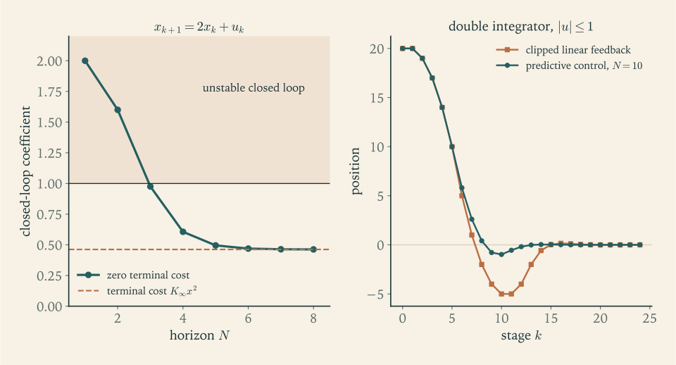
Let \(x_{k+1}=2x_k+u_k\) with \(\ell=x^{2}+4u^{2}\) and terminal cost \(F=0\) . The scalar recursion of Exercise 3.11 with \(a=2\) , \(b=1\) , \(q=1\) , \(r=4\) is \(K\mapsto1+\dfrac{16K}{4+K}\) , and the closed-loop coefficient under the gain built from \(K\) is \(2-L=\dfrac{8}{4+K}\) .
With \(N=1\) the gain is built from \(K=0\) : the controller sees no cost beyond the present stage that its control can affect, applies \(u=0\) , and the closed loop is \(x_{k+1}=2x_k\) . With \(N=2\) , \(K=1\) and the coefficient is \(\tfrac85=1.6\) . With \(N=3\) , \(K=4.2\) and the coefficient is \(0.976\) ; with \(N=4\) , \(K\approx9.195\) and it is \(0.606\) ; as \(N\to\infty\) it tends to \(0.462\) , the coefficient of the stationary regulator, for which \(K_\infty=\tfrac12(13+\sqrt{185})\approx13.30\) .
For \(N=1\) and \(N=2\) the closed loop is unstable, although at every step the controller solves its optimization problem exactly. With the terminal cost \(F=K_\infty x^{2}\) the coefficient is \(0.462\) at every horizon, including \(N=1\) .
The example shows what the terminal cost is for. It stands in for the cost of everything after the horizon, and a horizon that is too short with nothing at its end makes the controller blind to the consequences of an unstable state. The next theorem says which terminal costs are safe.
Theorem 10.4 (a terminal cost that guarantees decrease). Suppose the terminal cost is nonnegative and satisfies
Then \(V_N(x)\le V_{N-1}(x)\) for all \(x\) and \(N\ge1\) , where \(V_0=F\) , and along the closed loop \(x_{k+1}=f(x_k,\kappa_N(x_k))\) ,
Consequently the total closed-loop cost \(\sum_{k=0}^{\infty}\ell(x_k,\kappa_N(x_k))\) is at most \(V_N(x_0)\) .
Proof. Let \(\mathcal T\) denote the map \(V\mapsto\min_{u\in U}[\ell(\cdot,u)+V(f(\cdot,u))]\) . It is monotone, and \(V_N=\mathcal TV_{N-1}\) by the Bellman recursion. The hypothesis says \(V_1=\mathcal TF\le F=V_0\) . Applying \(\mathcal T\) repeatedly gives \(V_{N}\le V_{N-1}\) for every \(N\) . Now \(V_N(x_k)=\ell(x_k,\kappa_N(x_k))+V_{N-1}(x_{k+1})\ge\ell(x_k,\kappa_N(x_k))+V_N(x_{k+1})\) , which is the decrease inequality. Summing it from \(k=0\) to \(k=m\) gives \(\sum_{k=0}^{m}\ell\le V_N(x_0)-V_N(x_{m+1})\le V_N(x_0)\) , since \(V_N\ge0\) .
The condition says that \(F\) overestimates the cost of some admissible way of continuing, one stage at a time. A function \(V_N\) that decreases along trajectories by at least the stage cost forces the stage costs to be summable, and if \(\ell(x,u)\) is at least a positive multiple of \(\lvert x\rvert^{2}\) the state must tend to the origin. In Example 10.4 the terminal cost \(F=cx^{2}\) satisfies the condition exactly when \(c\ge K_\infty\) , and \(F=0\) fails it.
When the controls are constrained, the natural choice \(F(x)=x^{\top}K_\infty x\) satisfies the condition only for states small enough that the unconstrained optimal control is admissible. Practical schemes therefore either add a constraint that the predicted final state lie in such a region, or use a horizon long enough for it to do so unprompted, as in the next example.
Example 10.5: Constraints seen in advance
Take the double integrator of Example 3.5, with \(Q=\operatorname{diag}(1,0)\) and \(R=1\) , and add the constraint \(\lvert u_k\rvert\le1\) . Start from position \(20\) at rest. Two controllers are compared over a long run.
Clipped linear feedback. Apply the stationary regulator’s control \(-L_\infty x\) , clipped to \([-1,1]\) . From \((20,0)\) it pushes at full force toward the origin for five stages, by which time the cart is moving at speed \(5\) ; it then reverses, but cannot brake in time, and overshoots to position \(-5\) before returning. The total cost is \(1875.6\) .
Model predictive control with horizon \(N=10\) , terminal cost \(x^{\top}K_\infty x\) , and the constraint imposed on every predicted control. Each step solves a convex quadratic program in ten variables with bounds. The first four controls are \(-1\) ; the fifth is \(-0.196\) , and from the sixth the controller brakes at full force. It overshoots only to \(-0.98\) . The total cost is \(1797.1\) , lower by \(4.2\) percent.
The predictive controller eases off one stage earlier because its plan contains the braking phase and the bound on it. The clipped feedback was designed for a system with unlimited force and discovers the limit only when it hits it. With horizon \(N=5\) the predictive controller already attains \(1797.1\) , which is the exact optimum of the constrained problem; with \(N=3\) it attains \(1807.9\) , and with \(N=2\) it does no better than the clipped feedback.
Common mistake. Believing that because each step of model predictive control solves an optimal control problem, the closed loop inherits optimality or stability from it. The problem solved at each step is a different problem from the one the closed loop faces: it has a finite horizon, and only its first control is ever used. Example 10.4 shows an exact optimizer producing an unstable loop. What transfers from the finite-horizon problems to the closed loop is controlled by the terminal cost and the horizon, through results such as Theorem 10.4, and it has to be checked.
10.5 Learning the cost-to-go from simulation
All the methods so far used the model’s transition probabilities. When the model is available only as a simulator, or as a real system that can be observed, the Q-factor form of Bellman’s equation from Section 5.6 can be solved by averaging observed transitions. After observing a transition from state \(i\) under control \(u\) to state \(j\) at cost \(g\) , Q-learning updates one entry of a table:
with a small step size \(\gamma\) . The bracket is a single sample of the right side of the Q-factor equation, whose expectation is the exact right side. It can be shown that if every pair \((i,u)\) is updated infinitely often and the step sizes decrease at a suitable rate, the table converges to \(Q^\star\) ; the proof uses the contraction property together with the theory of stochastic approximation and is beyond this book. In large problems the table is replaced by a parametric function fitted to such samples. Then the contraction argument is no longer available in general, the approximation error \(\varepsilon\) of Theorem 10.1 is hard to bound, and performance is established by experiment. This is the territory of reinforcement learning, for which the present book supplies the foundations and no more.
10.6 The book as a single decision
The chapters of this book are answers to one question asked under different conditions: given a state, how should the control be chosen so that the cost from here on is small? The conditions that decide which answer applies are few.
| Feature of the problem | Tool | Where |
|---|---|---|
| Finite horizon, small finite state set | Backward induction | Chapter 2 |
| Deterministic, finite | Shortest path, forward or backward | Chapter 3 |
| Linear dynamics, quadratic cost, no constraints | Riccati recursion or equation | Chapters 3, 6, 9 |
| Infinite horizon, discounted, small state set | Value or policy iteration | Chapters 4, 5 |
| State not observed | Belief state, then the above | Chapter 7 |
| Only decision is when to stop | Threshold from the continuation value | Chapter 8 |
| Continuous time, one trajectory needed | Pontryagin conditions | Chapter 9 |
| Continuous time, feedback needed, low dimension | Hamilton–Jacobi–Bellman equation | Chapter 9 |
| Constraints, moderate dimension, good model | Model predictive control | Chapter 10 |
| State space too large for any table | Lookahead with an approximate cost-to-go | Chapter 10 |
Before any of these can be applied, the state has to be right, which is the business of Chapter 1 and, for policy classes, of Chapter 6.
Example 10.6: Four problems, four tools
A warehouse stocks one item, with stock between \(0\) and \(200\) , random demand, and a planning period of a year in weekly stages. The state is the stock: \(201\) values, \(52\) stages. Backward induction needs about \(52\cdot201\cdot201\) brackets, a trivial computation, and Theorem 6.6 suggests that the answer should have base-stock form, which gives a check on the output.
The same warehouse stocks six items that share a storage limit. The state has six components and \(201^{6}\approx6.6\times10^{13}\) values. A table is impossible. Candidates are a rollout of independent base-stock policies, using Section 10.2, or a relaxation of the shared limit to obtain a lower bound in the spirit of Section 6.3 against which heuristics can be judged.
A satellite’s attitude is to be held near a reference using reaction wheels with torque limits. Near the reference the dynamics are linear and the cost quadratic. With limits that are rarely active, the stationary regulator of Theorem 3.6 is the answer; if the limits are active often, model predictive control with the regulator’s \(K_\infty\) as terminal cost, as in Example 10.5.
A spacecraft is to be transferred between two orbits using the least propellant. One trajectory is wanted, from one known initial state, in a state space of dimension six or seven with a bounded thrust. This is the setting of Theorem 9.7. Where the switching function is not zero, the minimum condition gives a thrust that is at its limit or off, and the costate decides which. Where the switching function vanishes over an interval the condition is silent and the thrust may take intermediate values: a singular arc, as in Exercise 9.17, which does occur in practice, for instance in ascent through an atmosphere, and has to be examined separately. Either way the work is the solution of a two-point boundary value problem. A feedback law over the whole state space is neither needed nor obtainable.
In each case the choice was made by asking the questions in the table’s left column in order: what is the state and how large is its space, is there a formula, is feedback needed or a single trajectory, are there constraints. The methods are few; the judgment lies in the formulation.
That is also where the subject continues. Stochastic control in continuous time replaces the differential equation of Chapter 9 by a stochastic one and adds a second-order term to the Hamilton–Jacobi–Bellman equation; it needs the tools of Stochastic Calculus. Problems with several decision makers lead to Game Theory. And the approximate methods of this chapter, which here occupy a few pages, are a large and active field of their own.
Exercises
-
Define a one-step lookahead policy, a rollout policy, and a model predictive control law, and state the bound of Theorem 10.1 together with the role of each quantity in it.
Hint
A lookahead policy uses, in state \(i\) , a control attaining the minimum in \((T\tilde J)(i)\) for some approximation \(\tilde J\) . Rollout is the special case \(\tilde J=J_\mu\) for a base policy \(\mu\) . Model predictive control is the special case \(\tilde J=V_{N-1}\) , computed by an open-loop optimization from the current state. In the bound \(\tfrac{2\alpha\varepsilon}{1-\alpha}\) , \(\varepsilon\) is the error of \(\tilde J\) and \(\tfrac{1}{1-\alpha}\) is the effective horizon over which a repeated mistake accumulates.
-
For the three-state machine of Chapter 5 take \(\tilde J=(10,15,19)\) . Compute \(\varepsilon=\lVert\tilde J-J^\star\rVert\) , find the greedy policy for \(\tilde J\) by evaluating both brackets in each state, and compare its actual loss, using Example 10.1, with the bound of Theorem 10.1.
Solution
The error. \(J^\star=(10.630,\,14.567,\,19.110)\) , so the three errors of \(\tilde J=(10,15,19)\) are \(0.630\) , \(0.433\) , \(0.110\) in absolute value: \(\varepsilon=0.630\) .
The greedy policy. Good: run costs \(0.9\,(0.7\cdot10+0.3\cdot15)=10.35\) ; service costs \(1+0.9\,(0.95\cdot10+0.05\cdot15)=10.225\) . Service is smaller. Worn: run costs \(2+0.9\,(0.5\cdot15+0.5\cdot19)=17.3\) ; overhaul costs \(5+0.9\cdot10=14\) . Overhaul. Broken: replace costs \(12+9=21\) ; patch costs \(6+0.9\cdot15=19.5\) . Patch.
The greedy policy is (service, overhaul, patch), the policy of Example 10.1, whose cost is \((11.722,\,15.550,\,19.995)\) . Its loss is \(1.093\) .
The bound. Theorem 10.1 allows \(\dfrac{2\cdot0.9\cdot0.630}{0.1}\approx11.3\) . The actual loss is about a tenth of that. The bound must cover the worst arrangement of errors over all models, and here only one decision, the nearly indifferent one in the good state, was disturbed.
-
In a discounted model let \(\delta\) be the smallest difference, over all states, between the second-smallest and the smallest optimal Q-factor, and assume the minimizing control is unique in every state. Prove that if \(\lVert\tilde J-J^\star\rVert\le\varepsilon\) with \(2\alpha\varepsilon<\delta\) , then the greedy policy for \(\tilde J\) is optimal, and evaluate the threshold for the machine of Example 5.5.
Solution
Let \(\tilde Q(i,u)=g(i,u)+\alpha\sum_jp_{ij}(u)\tilde J(j)\) be the bracket that the greedy policy minimizes. For every pair,
\[ \big\lvert\tilde Q(i,u)-Q^\star(i,u)\big\rvert=\alpha\Big\lvert\sum_jp_{ij}(u)\big(\tilde J(j)-J^\star(j)\big)\Big\rvert\le\alpha\varepsilon, \]since the weights \(p_{ij}(u)\) are nonnegative and sum to \(1\) .
Fix a state \(i\) , let \(u^\star\) be its unique optimal control and \(u\) any other control. By the definition of \(\delta\) , \(Q^\star(i,u)-Q^\star(i,u^\star)\ge\delta\) . Then
\[ \tilde Q(i,u)-\tilde Q(i,u^\star)\ \ge\ \big(Q^\star(i,u)-\alpha\varepsilon\big)-\big(Q^\star(i,u^\star)+\alpha\varepsilon\big)\ \ge\ \delta-2\alpha\varepsilon, \]which is positive when \(2\alpha\varepsilon<\delta\) . So \(u^\star\) is the unique minimizer of \(\tilde Q(i,\cdot)\) , the greedy policy chooses it in every state, and the greedy policy is the optimal policy.
For the machine, the gaps in Example 5.5 are \(0.114\) , \(2.588\) , and \(2.457\) , so \(\delta=0.114\) , and the condition is \(\varepsilon<\dfrac{0.114}{1.8}\approx0.063\) . In Example 10.1 the error was \(0.3\) , well above this, and the policy changed. This result complements Theorem 10.1: the bound there degrades gracefully as \(\varepsilon\) grows, while this one says that below a threshold nothing is lost at all.
-
Apply the rollout algorithm to the staged network of Example 3.1, with the base heuristic “always take the shortest outgoing arc”. Give the heuristic’s path lengths from \(a_1\) and \(a_2\) , the choice rollout makes at \(s\) , and the length of the path rollout generates.
Solution
The heuristic. From \(a_1\) the shortest outgoing arc goes to \(b_2\) , length \(4\) ; from \(b_2\) to \(c_2\) , length \(3\) ; from \(c_2\) to \(t\) , length \(3\) . So \(\mathcal H(a_1)=10\) . From \(a_2\) the shortest arc goes to \(b_1\) , length \(3\) ; from \(b_1\) to \(c_1\) , length \(1\) ; then \(4\) to \(t\) . So \(\mathcal H(a_2)=8\) . The heuristic is sequentially consistent, because its choice at a node does not depend on how the node was reached.
Rollout at \(s\) . Compare \(2+\mathcal H(a_1)=12\) with \(3+\mathcal H(a_2)\) , that is, \(3+8=11\) . Rollout goes to \(a_2\) ; the heuristic itself would have gone to \(a_1\) .
Continuing. At \(a_2\) : to \(b_1\) costs \(3+\mathcal H(b_1)=3+5=8\) ; to \(b_2\) , \(4+6=10\) ; to \(b_3\) , \(4+\mathcal H(b_3)\) with \(\mathcal H(b_3)\) equal to \(7\) or \(6\) depending on the tie-break, in either case at least \(10\) . Go to \(b_1\) . At \(b_1\) : to \(c_1\) costs \(1+4=5\) , to \(c_2\) costs \(4+3=7\) . Go to \(c_1\) , then \(t\) .
Rollout generates \(s\to a_2\to b_1\to c_1\to t\) with length \(11\) , the shortest path found in Example 3.1, against \(12\) for the heuristic. One look ahead at the first node was enough to avoid the trap of the short first arc.
-
For the three-state machine of Chapter 5 with base policy (run, run, patch), identify the rollout policy and its cost vector from the computations of Example 5.3, and state which theorem guarantees that it is no worse than the base policy.
Answer
With base policy \(\mu^{0}=\) (run, run, patch), the rollout policy is the greedy policy for \(J_{\mu^{0}}\) , which Example 5.3 computed: (service, overhaul, replace), with cost \((11.722,\ 15.550,\ 22.550)\) against the base policy’s \((23.653,\ 32.414,\ 35.172)\) . Theorem 5.3 guarantees the improvement. The rollout policy is not optimal; a second step of policy iteration is needed for that.
-
A state has four components, each discretized to \(33\) values, and two control components, each discretized to \(9\) values. Count the state-control pairs examined in one sweep of value iteration, and the number of sweeps that could be done per day at \(10^{8}\) pairs per second.
Answer
\(33^{4}\cdot9^{2}=1{,}185{,}921\cdot81\approx9.6\times10^{7}\) pairs per sweep, about one second each at \(10^{8}\) pairs per second, so roughly \(90{,}000\) sweeps per day. One more state component would multiply the work per sweep by \(33\) .
-
In Example 10.3 with \(h=1\) , compute \(J(1)\) and \(J(2)\) by hand from the recursion and state the policy on the grid. Explain why the computed values can never be below the exact \(\phi x^{2}\) .
Answer
\(J(0)=0\) . \(J(1)\) : the control \(u=-1\) gives \(1+1+J(0)=2\) , and \(u=0\) would stay at \(1\) for ever at infinite cost, so \(J(1)=2\) . \(J(2)\) : \(u=-1\) gives \(4+1+J(1)=7\) and \(u=-2\) gives \(4+4+0=8\) , so \(J(2)=7\) . The policy is \(u=-1\) from positive states. Every control sequence available on the grid is available to the continuous problem, so the grid’s optimal cost cannot be below the continuous optimum \(\phi x^{2}\) , which is \(1.618\) and \(6.472\) at these two points.
-
For \(x_{k+1}=x_k+u_k\) with \(\ell=x^{2}+u^{2}\) and terminal cost \(F=0\) , find the model predictive control gain and the closed-loop coefficient for horizons \(N=1,2,3\) , and compare with the stationary regulator of Example 3.4.
Solution
With \(a=b=q=r=1\) the recursion is \(K\mapsto1+\dfrac{K}{1+K}\) and the gain built from \(K\) is \(L=\dfrac{K}{1+K}\) , with closed-loop coefficient \(1-L=\dfrac{1}{1+K}\) . Model predictive control with horizon \(N\) uses the first gain of an \(N\) -stage recursion started from \(K_N=0\) , that is, the gain built from the result of \(N-1\) steps.
\(N=1\) : built from \(K=0\) , so \(L=0\) and the coefficient is \(1\) . \(N=2\) : built from \(K=1\) , so \(L=\tfrac12\) and the coefficient is \(\tfrac12\) . \(N=3\) : built from \(K=\tfrac32\) , so \(L=\tfrac35\) and the coefficient is \(\tfrac25\) .
The coefficients are \(1\) , \(\tfrac12\) , \(\tfrac25\) , approaching \(\dfrac{1}{1+\phi}\approx0.382\) , the coefficient of the stationary regulator with \(L_\infty\approx0.618\) . With \(N=1\) the controller does nothing and the state stays where it is: the system is not unstable, since \(a=1\) , but it is not regulated either. Two stages of lookahead already give a contraction by one half.
-
For \(x_{k+1}=3x_k+u_k\) with \(\ell=x^{2}+u^{2}\) and \(F=0\) , find the smallest horizon \(N\) for which model predictive control gives a stable closed loop.
Solution
By Exercise 3.11 with \(a=3\) , \(b=q=r=1\) , the Riccati map is \(K\mapsto1+\dfrac{9K}{1+K}\) , the gain built from \(K\) is \(L=\dfrac{3K}{1+K}\) , and the closed-loop coefficient is \(3-L=\dfrac{3}{1+K}\) . Model predictive control with horizon \(N\) and no terminal cost uses the gain built from the result of \(N-1\) applications of the map to \(0\) (Theorem 10.3).
\(N=1\) : \(K=0\) , coefficient \(3\) . The controller applies no control and the state triples at each step.
\(N=2\) : \(K=1\) , coefficient \(\tfrac32\) . Still unstable.
\(N=3\) : \(K=1+\tfrac92=5.5\) , coefficient \(\tfrac{3}{6.5}\approx0.46\) . Stable.
The smallest stabilizing horizon is \(N=3\) . The closed loop is stable when \(\dfrac{3}{1+K}\) is less than \(1\) , that is, when the terminal weight seen by the first control exceeds \(2\) ; the first two values of \(K\) , \(0\) and \(1\) , are too small, and the third is not. The more unstable the plant, the more a short-sighted controller underestimates the cost of leaving the state where it is.
-
Prove the first claim of Theorem 10.4 in detail: that the map \(\mathcal T\) is monotone, and that \(\mathcal TF\le F\) implies \(V_N\le V_{N-1}\) for all \(N\ge1\) .
Solution
Monotonicity. Let \(V\le V'\) pointwise. For each state \(x\) and each \(u\in U\) , \(V(f(x,u))\le V'(f(x,u))\) , so \(\ell(x,u)+V(f(x,u))\le\ell(x,u)+V'(f(x,u))\) . Let \(u'\) attain the minimum of the right side over \(U\) . Then
\[ (\mathcal TV)(x)\le\ell(x,u')+V(f(x,u'))\le\ell(x,u')+V'(f(x,u'))=(\mathcal TV')(x). \]So \(\mathcal TV\le\mathcal TV'\) . If the minimum is not attained the same argument works with an infimum and a control within any tolerance of it.
The chain. By the Bellman recursion for the \(N\) -stage problem, \(V_N=\mathcal TV_{N-1}\) with \(V_0=F\) . The hypothesis \(\min_u[\ell(x,u)+F(f(x,u))]\le F(x)\) says exactly that \(V_1=\mathcal TF\le F=V_0\) . Suppose \(V_N\le V_{N-1}\) for some \(N\ge1\) . Applying the monotone map \(\mathcal T\) to both sides gives \(V_{N+1}=\mathcal TV_N\le\mathcal TV_{N-1}=V_N\) . By induction \(V_N\le V_{N-1}\) for every \(N\ge1\) .
The meaning is that a longer horizon can only lower the predicted cost, because the terminal cost was pessimistic: one more stage of optimized control, followed by the same terminal cost, costs no more than the terminal cost alone. Without the hypothesis the sequence \(V_N\) need not be monotone at all; with \(F=0\) and nonnegative stage costs it is increasing instead.
-
An engineer says: “At every sampling instant my controller computes the exact optimal control sequence for the next two steps, so the closed loop is optimal and in particular stable.” Use Example 10.4 to refute the claim and say what additional design element would justify a stability conclusion.
Answer
Example 10.4 with \(N=2\) is exactly this situation: the two-step problem is solved exactly at every instant and the closed loop is \(x_{k+1}=1.6\,x_k\) , which diverges. Optimality of each finite-horizon plan says nothing about the infinite-horizon behaviour of applying only first controls. A terminal cost satisfying the condition of Theorem 10.4, such as \(K_\infty x^{2}\) , or a sufficiently long horizon, is what justifies a stability claim.
-
A value function is known to within \(1\) percent, in the sense that \(\lVert\tilde J-J^\star\rVert\le0.01\,\lVert J^\star\rVert\) , in a problem with \(\alpha=0.99\) . A colleague concludes that the greedy policy is within \(1\) percent of optimal. State what Theorem 10.1 actually guarantees and explain the discrepancy.
Answer
Theorem 10.1 guarantees \(\lVert J_{\tilde\mu}-J^\star\rVert\le\dfrac{2\cdot0.99}{0.01}\cdot0.01\,\lVert J^\star\rVert=1.98\,\lVert J^\star\rVert\) : a loss of up to \(198\) percent, not \(1\) percent. The factor \(\tfrac{2\alpha}{1-\alpha}=198\) reflects the possibility that a wrong control is repeated over an effective horizon of \(100\) stages. The actual loss is often far smaller, as Exercise 3 explains, but the guarantee is what it is.
-
For \(x_{k+1}=x_k+u_k\) with \(\lvert u_k\rvert\le1\) , \(\ell=x^{2}+u^{2}\) , horizon \(N=1\) , and terminal cost \(F(x)=\phi x^{2}\) with \(\phi=\tfrac12(1+\sqrt5)\) , find the model predictive control law as an explicit function of \(x\) , and simulate it from \(x_0=3\) for four steps.
Solution
With \(N=1\) the controller minimizes \(x^{2}+u^{2}+\phi\,(x+u)^{2}\) over \(u\in[-1,1]\) . This is a convex function of one variable. Its unconstrained minimizer satisfies \(2u+2\phi(x+u)=0\) , so \(u=-\dfrac{\phi}{1+\phi}x\) . Since \(\phi^{2}=\phi+1\) , \(\dfrac{\phi}{1+\phi}=\dfrac1\phi\approx0.618\) : this is the stationary gain \(L_\infty\) of Example 3.4, as Theorem 10.3 predicts for the terminal cost \(K_\infty=\phi\) . A convex function of one variable is minimized over an interval at the point of the interval closest to its unconstrained minimizer, so
\[ \kappa_1(x)=\max\big\{-1,\ \min\{1,\ -0.618\,x\}\big\}. \]From \(x_0=3\) : \(-0.618\cdot3=-1.854\) is clipped to \(-1\) , giving \(x_1=2\) ; \(-1.236\) is clipped to \(-1\) , giving \(x_2=1\) ; \(u=-0.618\) gives \(x_3=0.382\) ; \(u=-0.236\) gives \(x_4=0.146\) . The states are \(3,\ 2,\ 1,\ 0.382,\ 0.146\) .
In this scalar problem with a one-step horizon, model predictive control coincides with clipping the linear feedback. The two differ, as in Example 10.5, when the horizon is longer and the state has more than one component, so that the best response to a future saturation is to act differently now.
-
A Q-learning table has \(Q(1,\text{run})=4\) , \(Q(2,\text{run})=7\) , and \(Q(2,\text{overhaul})=6\) . A transition is observed from state \(1\) under “run” to state \(2\) at cost \(0\) . With \(\alpha=0.9\) and step size \(\gamma=0.1\) , compute the updated entry and say which entries are unchanged.
Answer
The sample is \(g+\alpha\min_vQ(2,v)=0+0.9\cdot6=5.4\) . The update gives \(Q(1,\text{run})=0.9\cdot4+0.1\cdot5.4=4.14\) . The entries for state \(2\) are unchanged; only the entry of the pair that was visited moves.
-
For each problem name the tool from the table of Section 10.6 and the state you would use: (a) deciding each day whether to sell a perishable asset whose price follows a known Markov chain; (b) steering a ship along a prescribed track with rudder-angle limits; (c) scheduling maintenance for a machine whose wear can only be inferred from vibration readings; (d) finding the cheapest route through a road network with known travel times.
Hint
(a) A stopping problem: the state is the current price, with the day if there is a deadline; compare stopping with the continuation value. (b) Linear dynamics near the track, quadratic deviation cost, and a constraint that is often active: model predictive control with the regulator’s terminal cost; the state is the track error and heading. (c) Partial observation: the state is the belief about the wear. (d) Deterministic and finite: a shortest path, with the junction as the state.
-
Apply the receding-horizon idea to Example 9.1: at every instant use the control that is optimal for a horizon of fixed length \(T\) starting now, which gives the feedback \(u=-\tanh(T)\,x\) . Compute the infinite-horizon cost \(\int_0^{\infty}(x^{2}+u^{2})\,dt\) of this feedback from \(x_0=1\) as a function of \(T\) , evaluate it for \(T=0.5\) and \(T=2\) , and compare with the optimal infinite-horizon cost.
Solution
Write \(\tau=\tanh T\) . The feedback \(u=-\tau x\) gives \(\dot x=-\tau x\) , so \(x(t)=e^{-\tau t}\) from \(x_0=1\) , and
\[ \int_0^{\infty}(x^{2}+u^{2})\,dt=(1+\tau^{2})\int_0^{\infty}e^{-2\tau t}\,dt=\frac{1+\tau^{2}}{2\tau}. \]The optimal infinite-horizon feedback is \(u=-x\) , by the stationary Riccati equation \(K^{2}=1\) , with cost \(1\) ; this is the case \(\tau=1\) , and indeed \(\tfrac{1+\tau^{2}}{2\tau}\ge1\) with equality only at \(\tau=1\) .
For \(T=0.5\) , \(\tau\approx0.4621\) and the cost is \(1.313\) , a loss of \(31\) percent. For \(T=2\) , \(\tau\approx0.9640\) and the cost is \(1.0007\) .
The receding-horizon controller with a short horizon and no terminal cost under-controls, because the plan it solves at each instant ends with a stretch in which control is not worth applying, and it is always at the start of such a plan. Lengthening the horizon to a few time constants, or adding the terminal cost \(x^{2}\) , which by Exercise 9.5 makes the gain exactly \(1\) for every \(T\) , removes the loss. This is the continuous-time picture of Example 10.4.
-
Show that the nearest-neighbour heuristic of Example 10.2, with a fixed rule for breaking ties, is sequentially consistent, and verify the conclusion of Proposition 10.2 for the starting city A using the numbers of that example.
Hint
The heuristic’s next city depends only on the current city and the set of cities already visited. After the heuristic moves from a partial tour to the next city, it faces exactly the situation it would face if started from the extended partial tour, so it continues along the same path: that is sequential consistency. For city A: \(\mathcal H=21\) and \(\mathcal R=19\) , so \(\mathcal R\le\mathcal H\) .
-
Suppose value iteration is carried out inexactly, so that \(\lVert J_{k+1}-TJ_k\rVert\le\delta\) for every \(k\) . Prove that \(\limsup_{k\to\infty}\lVert J_k-J^\star\rVert\le\dfrac{\delta}{1-\alpha}\) , and combine this with Theorem 10.1 to bound the loss of the greedy policy for a late iterate.
Solution
Let \(e_k=\lVert J_k-J^\star\rVert\) . By the triangle inequality, the hypothesis, and the contraction property with \(TJ^\star=J^\star\) ,
\[ e_{k+1}\le\lVert J_{k+1}-TJ_k\rVert+\lVert TJ_k-TJ^\star\rVert\le\delta+\alpha\,e_k . \]Iterating, \(e_k\le\alpha^{k}e_0+\delta\,(1+\alpha+\dots+\alpha^{k-1})\le\alpha^{k}e_0+\dfrac{\delta}{1-\alpha}\) . The first term tends to zero, so \(\limsup_{k\to\infty}e_k\le\dfrac{\delta}{1-\alpha}\) .
For the policy: fix any \(\eta\) greater than \(0\) . For all large \(k\) , \(e_k\le\dfrac{\delta}{1-\alpha}+\eta\) , and Theorem 10.1 with this value of \(\varepsilon\) bounds the loss of the greedy policy for \(J_k\) by \(\dfrac{2\alpha}{1-\alpha}\Big(\dfrac{\delta}{1-\alpha}+\eta\Big)\) . Since \(\eta\) is arbitrary, the loss of the greedy policy for a late iterate is at most, in the limit, \(\dfrac{2\alpha\,\delta}{(1-\alpha)^{2}}\) .
The square of the effective horizon appears: one factor because a per-iteration error accumulates over about \(\tfrac1{1-\alpha}\) iterations before the contraction damps it, and another because a wrong decision is repeated over about \(\tfrac1{1-\alpha}\) stages. With \(\alpha=0.99\) a per-iteration error of \(10^{-3}\) can cost up to about \(20\) . This is why approximate value iteration with a fitted function is delicate when the discount factor is close to \(1\) .