Bellman’s equation \(J=TJ\) is a system of \(n\) equations, one per state, and each contains a minimum. It cannot be solved by elimination. In Example 4.3 the system was solved by guessing the right policy and checking; with two policies that was easy, but a model with \(n\) states and \(m\) controls has \(m^{n}\) stationary policies.
Two ideas turn the theory of Chapter 4 into computation. The first is to iterate \(T\) : the contraction property guarantees convergence, slowly when \(\alpha\) is close to \(1\) . The second is to alternate between two easy problems: computing the cost of a fixed policy, which is linear, and choosing the best control in each state against a fixed cost function, which is a separate small minimization for each state. This chapter develops both methods, proves what each guarantees, runs them side by side on one machine-maintenance problem, and looks closely at a question that matters in practice: when the iteration is stopped early, how wrong can the answer be?
The running example extends the machine of Chapter 4. The machine is good, worn, or broken (states \(1,2,3\) ), and \(\alpha=0.9\) .
| State | Control | Cost | Next state |
|---|---|---|---|
| good | run | \(0\) | good with probability \(0.7\) , worn \(0.3\) |
| good | service | \(1\) | good \(0.95\) , worn \(0.05\) |
| worn | run | \(2\) | worn \(0.5\) , broken \(0.5\) |
| worn | overhaul | \(5\) | good |
| broken | replace | \(12\) | good |
| broken | patch | \(6\) | worn |
There are \(2^{3}=8\) stationary policies. A policy is written as a triple, such as (run, overhaul, patch).
5.1 Value iteration and the question of when to stop
Value iteration chooses any \(J_0\) and computes \(J_{k+1}=TJ_k\) . By Theorem 4.5, \(\lVert J_k-J^\star\rVert\le\alpha^{k}\lVert J_0-J^\star\rVert\) . Each iteration costs one bracket per pair of state and control. When the iteration is stopped, the policy that is greedy with respect to the last iterate, meaning \(T_\mu J_k=TJ_k\) , is the natural output.
Example 5.1: Value iteration on the three-state machine
Start from \(J_0=(0,0,0)\) . The first iterate is the vector of smallest one-stage costs, \(J_1=(0,2,6)\) , with greedy policy (run, run, patch): the cheapest control in each state. For the second,
\(J_2(2)=\min\{2+0.9\cdot4,\ 5+0\}=5\) , and \(J_2(3)=\min\{12+0,\ 6+0.9\cdot2\}=7.8\) . Continuing:
| \(k\) | \(J_k(1)\) | \(J_k(2)\) | \(J_k(3)\) | policy greedy for \(J_{k-1}\) | \(\lVert J_k-J^\star\rVert\) |
|---|---|---|---|---|---|
| \(1\) | \(0\) | \(2\) | \(6\) | (run, run, patch) | \(13.110\) |
| \(2\) | \(0.54\) | \(5\) | \(7.8\) | (run, overhaul, patch) | \(11.310\) |
| \(3\) | \(1.6867\) | \(5.486\) | \(10.5\) | (service, overhaul, patch) | \(9.081\) |
| \(4\) | \(2.5438\) | \(6.5180\) | \(10.9374\) | (run, overhaul, patch) | \(8.173\) |
| \(5\) | \(3.3625\) | \(7.2895\) | \(11.8662\) | (run, overhaul, patch) | \(7.277\) |
| \(10\) | \(6.3372\) | \(10.2742\) | \(14.8175\) | (run, overhaul, patch) | \(4.293\) |
The last column uses the exact solution \(J^\star=(10.630,\,14.567,\,19.110)\) , which Example 5.3 will obtain. From \(k=4\) on the greedy policy no longer changes, and it is the optimal one. The values are another matter: at \(k=10\) they are still off by more than \(4\) , and it takes \(155\) iterations to bring the error below \(10^{-6}\) . The error shrinks by the factor \(0.9\) per iteration almost exactly, so the bound of Theorem 4.5 is tight here.
In practice \(J^\star\) is not available to measure the error against. What is available is the size of the last step.
Proposition 5.1 (a stopping rule). For value iteration, for every \(k\ge1\) ,
Proof. By the triangle inequality and Proposition 4.4 applied twice,
Moving the last term to the left and dividing by \(1-\alpha\) gives the claim.
Common mistake. Stopping when two successive iterates agree to within a tolerance and reporting that tolerance as the accuracy. The proposition shows the true guarantee is larger by the factor \(\dfrac{\alpha}{1-\alpha}\) , which is \(9\) for \(\alpha=0.9\) and \(999\) for \(\alpha=0.999\) . In Example 5.1 the step from \(J_9\) to \(J_{10}\) has size \(0.477\) , and the error of \(J_{10}\) is \(4.293=9\cdot0.477\) . Small steps mean slow progress, not arrival.
5.2 Bounds that are better than the iterate
Example 5.1 contains a puzzle. The greedy policy was already optimal at \(k=4\) , when the values were wrong by \(8\) . How can a badly wrong cost vector produce the right policy?
Look at the iterates: from one row to the next, all three components increase by nearly the same amount. The error \(J_k-J^\star\) is close to a constant vector, and adding a constant to \(J\) changes no comparison between controls, because by Lemma 4.3 it adds the same amount to every bracket. The iterate is poor as an estimate of the level of \(J^\star\) and good as an estimate of its shape. The next result extracts the level.
Proposition 5.2 (two-sided error bounds). For value iteration and \(k\ge1\) let
Then \(J_k+\underline c_k\mathbf 1\le J^\star\le J_k+\overline c_k\mathbf 1\) .
Proof. Let \(\delta=\min_i[J_k(i)-J_{k-1}(i)]\) , so that \(J_{k-1}+\delta\mathbf 1\le J_k\) . Applying \(T\) and using Lemma 4.3 gives \(J_k+\alpha\delta\mathbf 1\le J_{k+1}\) . Applying \(T\) again gives \(J_{k+1}+\alpha^{2}\delta\mathbf 1\le J_{k+2}\) , and in general \(J_{k+m-1}+\alpha^{m}\delta\mathbf 1\le J_{k+m}\) . Adding these inequalities for \(m=1,\dots,r\) ,
Let \(r\to\infty\) : the right side tends to \(J^\star\) and the sum to \(\dfrac{\alpha}{1-\alpha}\) . That is the lower bound; the upper bound is the same argument with the maximum and reversed inequalities.
Example 5.2: Ten iterations are enough
In Example 5.1, \(J_{10}-J_9=(0.47695,\ 0.47702,\ 0.47679)\) . The three increments agree to three decimal places, as the discussion above predicted. With \(\dfrac{\alpha}{1-\alpha}=9\) the bounds are
The exact \(J^\star=(10.6299,\,14.5669,\,19.1102)\) lies between them, and the gap between the bounds is \(0.002\) . The raw iterate \(J_{10}\) was off by \(4.3\) . After five iterations the same computation gives a gap of \(1.42\) ; after ten, \(0.002\) .
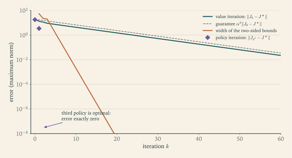
The steep line in Figure 5.1 has a reason. The component of the error along the constant vector is the slowest to die, at rate \(\alpha\) , because constants are exactly what the transition matrix preserves. The bounds of Proposition 5.2 are insensitive to that component, and what remains decays at a rate governed by how fast the Markov chain of the optimal policy forgets its initial state.
5.3 Evaluating a fixed policy
By Theorem 4.5 the cost of a stationary policy solves the linear system
with an invertible matrix (Exercise 4.5). Two routes are available. A direct solve by elimination costs of order \(n^{3}\)
operations and gives the exact answer; methods and their reliability are the subject of Numerical Analysis (math.numerical-analysis.linear-systems). Alternatively, iterate \(J\leftarrow T_\mu J=g_\mu+\alpha P_\mu J\)
, which costs of order \(n^{2}\)
per sweep, fewer if \(P_\mu\)
is sparse, and converges at rate \(\alpha\)
. For small models the direct solve is the obvious choice; for very large sparse ones only the iteration is feasible.
5.4 Improving a policy
The failed test in Example 4.3 pointed to a better policy. That was no accident.
Theorem 5.3 (policy improvement). Let \(\mu\) be a stationary policy and let \(\bar\mu\) be greedy with respect to \(J_\mu\) , that is, \(T_{\bar\mu}J_\mu=TJ_\mu\) . Then \(J_{\bar\mu}\le J_\mu\) . If \(\mu\) is not optimal, then \(J_{\bar\mu}(i)\) is strictly less than \(J_\mu(i)\) for at least one state \(i\) .
Proof. Since \(J_\mu=T_\mu J_\mu\ge TJ_\mu=T_{\bar\mu}J_\mu\) , we have \(T_{\bar\mu}J_\mu\le J_\mu\) . Applying the monotone operator \(T_{\bar\mu}\) repeatedly gives
the limit by Theorem 4.5. So \(J_{\bar\mu}\le T_{\bar\mu}J_\mu=TJ_\mu\le J_\mu\) . If \(J_{\bar\mu}=J_\mu\) , the chain of inequalities forces \(J_\mu=TJ_\mu\) , so \(J_\mu=J^\star\) by Theorem 4.6 and \(\mu\) is optimal. Hence if \(\mu\) is not optimal the two cost vectors differ, and since \(J_{\bar\mu}\le J_\mu\) the difference is strict in some state.
Policy iteration repeats the two steps. Start from any stationary policy \(\mu^{0}\) . At iteration \(k\) : evaluate, solving \((I-\alpha P_{\mu^{k}})J=g_{\mu^{k}}\) for \(J_{\mu^{k}}\) ; then improve, choosing \(\mu^{k+1}\) greedy with respect to \(J_{\mu^{k}}\) , keeping \(\mu^{k+1}(i)=\mu^{k}(i)\) whenever the current control is among the minimizers. Stop when \(\mu^{k+1}=\mu^{k}\) .
Theorem 5.4 (policy iteration terminates). Policy iteration stops after finitely many iterations, and the policy at which it stops is optimal. Moreover, for every \(k\) before termination, \(\lVert J_{\mu^{k+1}}-J^\star\rVert\le\alpha\,\lVert J_{\mu^{k}}-J^\star\rVert\) .
Proof. If \(\mu^{k+1}=\mu^{k}\) , then \(T_{\mu^{k}}J_{\mu^{k}}=TJ_{\mu^{k}}\) , so \(J_{\mu^{k}}=TJ_{\mu^{k}}\) and \(\mu^{k}\) is optimal by Theorem 4.6. If \(\mu^{k+1}\ne\mu^{k}\) , the tie-breaking rule means that \(\mu^{k}\) was not greedy with respect to its own cost, so \(J_{\mu^k}\ne TJ_{\mu^k}\) and \(\mu^{k}\) is not optimal; by Theorem 5.3, \(J_{\mu^{k+1}}\le J_{\mu^{k}}\) with strict inequality somewhere. The cost vectors therefore strictly decrease along the iteration, no policy can occur twice, and there are finitely many policies.
For the rate: the proof of Theorem 5.3 showed \(J_{\mu^{k+1}}\le TJ_{\mu^{k}}\) , and \(J^\star\le J_{\mu^{k+1}}\) . Hence \(0\le J_{\mu^{k+1}}-J^\star\le TJ_{\mu^{k}}-TJ^\star\) , and the right side has norm at most \(\alpha\lVert J_{\mu^{k}}-J^\star\rVert\) .
The last statement says that one policy iteration step gains at least as much as one value iteration step from the same starting point. In practice it gains far more.
Example 5.3: Policy iteration from the myopic policy
Start from \(\mu^{0}=\) (run, run, patch), the policy that minimizes the immediate cost in each state.
Evaluate \(\mu^{0}\) . The equations are \(J(1)=0.9\,(0.7J(1)+0.3J(2))\) , \(J(2)=2+0.9\,(0.5J(2)+0.5J(3))\) , \(J(3)=6+0.9J(2)\) . Substituting the third into the second, \(0.55J(2)=2+0.45\,(6+0.9J(2))\) , so \(0.145J(2)=4.7\) :
Improve. Compute both brackets in each state with this \(J\) . Good: run \(23.653\) , service \(1+0.9\,(0.95\cdot23.653+0.05\cdot32.414)=22.682\) . Worn: run \(32.414\) , overhaul \(5+0.9\cdot23.653=26.288\) . Broken: patch \(35.172\) , replace \(12+0.9\cdot23.653=33.288\) . Every state switches: \(\mu^{1}=\) (service, overhaul, replace).
Evaluate \(\mu^{1}\) . Solving the new linear system gives \(J_{\mu^{1}}=(11.722,\ 15.550,\ 22.550)\) , which halves the cost from the good and worn states.
Improve. Good: run \(0.9\,(0.7\cdot11.722+0.3\cdot15.550)=11.584\) , service \(11.722\) . Worn: run \(2+0.9\cdot\tfrac12(15.550+22.550)=19.145\) , overhaul \(15.550\) . Broken: replace \(22.550\) , patch \(6+0.9\cdot15.550=19.995\) . Two states switch: \(\mu^{2}=\) (run, overhaul, patch).
Evaluate \(\mu^{2}\) . The good and worn states now form the two-state machine of Example 4.1, so \(J(1)=\tfrac{1350}{127}\) and \(J(2)=\tfrac{1850}{127}\) , and \(J(3)=6+0.9J(2)=\tfrac{2427}{127}\) :
Improve. Good: run \(10.630\) , service \(10.744\) . Worn: run \(17.155\) , overhaul \(14.567\) . Broken: replace \(21.567\) , patch \(19.110\) . Nothing switches, so \(\mu^{2}\) is optimal and \(J^\star=J_{\mu^{2}}\) .
Three linear solves of size \(3\) produced the exact answer, against \(155\) sweeps of value iteration for six-digit accuracy. The first improvement over-corrected: fearing the expensive broken state under the myopic policy, it serviced the good machine and replaced the broken one. Once the worn machine is overhauled, the broken state is never visited from good or worn, servicing is not worth its cost, and a cheap patch suffices if the machine is ever found broken.
Policy iteration is Newton’s method applied to the equation \(J-TJ=0\)
: the evaluation step solves the equation linearized at the current policy. That explains its fast convergence near the solution, and Newton’s method is analysed in Numerical Analysis (math.numerical-analysis.newton-fixed-point).
5.5 Between the two methods
Policy iteration spends heavily on each evaluation; value iteration spends almost nothing and makes almost no progress per step. Two variations sit between them.
Modified policy iteration replaces the exact evaluation by a fixed number of sweeps: from \(J_k\) , find the greedy policy \(\mu\) , then set \(J_{k+1}=T_\mu^{m}J_k\) . With \(m=1\) this is value iteration, since \(T_\mu J_k=TJ_k\) ; as \(m\to\infty\) it becomes policy iteration. The minimization over controls, which is the expensive part when there are many controls, is done once per \(m\) sweeps.
Gauss–Seidel value iteration updates the states one at a time and uses each new value at once: when \(J(i)\) is recomputed, the values \(J(1),\dots,J(i-1)\) already computed in the current sweep are used in the bracket. It needs no second array and typically converges in fewer sweeps.
Example 5.4: Counting sweeps
For the three-state machine, starting from zero and stopping when the error is below \(10^{-6}\) : value iteration needs \(155\) sweeps, each with a minimization. Modified policy iteration with \(m=5\) needs \(31\) outer iterations, that is, \(31\) minimizations and \(155\) sweeps in all; with \(m=10\) it needs \(16\) minimizations. Gauss–Seidel value iteration needs \(122\) sweeps. Policy iteration needed \(3\) linear solves.
For this tiny model the comparison is academic. It stops being so when a sweep costs minutes. The ordering by number of minimizations, policy iteration first, then modified policy iteration, then value iteration, is typical; so is the fact that the total number of sweeps in modified policy iteration hardly depends on \(m\) , because sweeps of either kind contract at rate \(\alpha\) .
5.6 Q-factors
Define the optimal Q-factor of a state-control pair, as in Chapter 2, by
Then \(J^\star(i)=\min_uQ^\star(i,u)\) , and substituting this into the definition shows that \(Q^\star\) satisfies an equation of its own,
whose right side defines a contraction on functions of pairs \((i,u)\) , by the argument of Proposition 4.4. Value iteration can therefore be run on Q-factors. It needs more memory, one number per pair in place of one per state. Its advantage is that the optimal control in state \(i\) is the minimizer of \(Q^\star(i,\cdot)\) and can be found without the model: no transition probabilities are needed once the Q-factors are known. That is the basis of the simulation-based methods mentioned in Chapter 10.
Example 5.5: What a mistake costs
From the last improvement step of Example 5.3, the optimal Q-factors of the machine are
| State | Control | \(Q^\star\) | Excess over \(J^\star\) |
|---|---|---|---|
| good | run | \(10.630\) | \(0\) |
| good | service | \(10.744\) | \(0.114\) |
| worn | run | \(17.155\) | \(2.588\) |
| worn | overhaul | \(14.567\) | \(0\) |
| broken | replace | \(21.567\) | \(2.457\) |
| broken | patch | \(19.110\) | \(0\) |
The last column is the loss from using the wrong control once and behaving optimally afterwards. Servicing a good machine is nearly harmless. Running a worn machine is the costly error, about \(18\) percent of the cost-to-go from that state. A table of Q-factors ranks the decisions by how much care they deserve, which the optimal policy alone does not.
5.7 Linear programming
There is a third route to \(J^\star\) , which uses no iteration designed for this problem at all.
Proposition 5.5 (linear programming formulation). \(J^\star\) is the unique optimal solution of the linear program
Proof. The constraints say exactly that \(J\le TJ\) . By Exercise 4.13 every such \(J\) satisfies \(J\le J^\star\) , so \(\sum_iJ(i)\le\sum_iJ^\star(i)\) . And \(J^\star\) is itself feasible, since \(J^\star=TJ^\star\) . So \(J^\star\) is optimal. Any other optimal solution \(J\) has \(J\le J^\star\) with equal sums, which forces equality in every component.
The program has \(n\)
variables and one constraint per pair of state and control. The theory of linear programs, their duals, and the simplex method belongs to Continuous Optimization (math.continuous-optimization.linear-programming-vertices-duality). At the solution, the constraints that hold with equality in state \(i\)
identify the optimal controls there.
Example 5.6: The machine as a linear program
For the three-state machine the program is: maximize \(J(1)+J(2)+J(3)\) subject to
A linear programming solver returns \(J=(10.630,\ 14.567,\ 19.110)\) . The first constraint of the first row, the second of the second row, and the second of the third row are active, which are the controls run, overhaul, and patch.
5.8 Choosing a method
For a model small enough that an \(n\times n\) linear system can be solved directly, policy iteration is hard to beat: it is exact and takes a handful of iterations, rarely more than a few dozen whatever \(n\) is. When \(n\) is in the millions, direct solves are out of reach, and value iteration or modified policy iteration with sparse sweeps is used, with the bounds of Proposition 5.2 as the stopping test. When \(\alpha\) is very close to \(1\) , plain value iteration is slow and the two-sided bounds, or policy iteration, matter most. Linear programming is seldom the fastest, but it accepts extra linear constraints on the policy’s long-run behaviour that the other methods cannot handle.
All of these assume that the state is known when the control is chosen and that the model’s probabilities are the true ones. Chapter 6 looks hard at the first assumption: what the controller knows, when, and what difference it makes.
Exercises
-
Describe value iteration and policy iteration in a few sentences each, and state for each what one iteration costs in a model with \(n\) states and \(m\) controls per state, and what is guaranteed about the error after \(k\) iterations.
Hint
Value iteration: \(J_{k+1}=TJ_k\) , one bracket per state-control pair, so of order \(n^{2}m\) operations per iteration for dense transitions, with error at most \(\alpha^{k}\lVert J_0-J^\star\rVert\) . Policy iteration: one linear solve, of order \(n^{3}\) , plus one improvement step, of order \(n^{2}m\) ; the error contracts at least by \(\alpha\) per iteration and the method stops at an optimal policy after finitely many iterations.
-
For the three-state machine of this chapter, apply \(T\) once to \(J=(10,15,20)\) , listing both brackets in each state, and state the greedy policy.
Answer
Good: run \(0.9\,(0.7\cdot10+0.3\cdot15)=10.35\) , service \(1+0.9\,(0.95\cdot10+0.05\cdot15)=10.225\) . Worn: run \(2+0.9\,(0.5\cdot15+0.5\cdot20)=17.75\) , overhaul \(5+0.9\cdot10=14\) . Broken: replace \(12+9=21\) , patch \(6+0.9\cdot15=19.5\) . So \(TJ=(10.225,\ 14,\ 19.5)\) and the greedy policy is (service, overhaul, patch).
-
Apply policy iteration to the two-state machine of Example 4.1, starting from “never overhaul”. Show the evaluation, the improvement step with both brackets in state \(2\) , the second evaluation, and the test that stops the algorithm.
Solution
Evaluate \(\mu^{0}\) , “never overhaul”. From Example 4.1, \(J_{\mu^{0}}=\big(\tfrac{540}{37},\,20\big)\approx(14.595,\,20)\) .
Improve. State \(1\) has one control. In state \(2\) the brackets with \(J_{\mu^{0}}\) are: run, \(2+0.9\cdot20=20\) ; overhaul, \(5+0.9\cdot14.595=18.135\) . The smaller is overhaul, so \(\mu^{1}\) is “overhaul when worn”. The policy has changed, so continue.
Evaluate \(\mu^{1}\) . From Example 4.1, \(J_{\mu^{1}}=\big(\tfrac{1350}{127},\tfrac{1850}{127}\big)\approx(10.630,\,14.567)\) . As Theorem 5.3 promises, both components have decreased.
Improve. In state \(2\) : run, \(2+0.9\cdot14.567=15.110\) ; overhaul, \(5+0.9\cdot10.630=14.567\) . The current control, overhaul, attains the minimum, so \(\mu^{2}=\mu^{1}\) and the algorithm stops. By Theorem 5.4 “overhaul when worn” is optimal and \(J^\star=(10.630,\,14.567)\) .
Two evaluations and two improvement steps were needed, and the stopping test is the Bellman test of Example 4.3: policy iteration stops exactly when the current policy’s cost satisfies Bellman’s equation.
-
Value iteration with \(\alpha=0.95\) is stopped when \(\lVert J_k-J_{k-1}\rVert\le0.01\) . What accuracy does Proposition 5.1 guarantee for \(J_k\) ? How small must the step be to guarantee an error of at most \(0.01\) ?
Answer
\(\dfrac{\alpha}{1-\alpha}=19\) , so the guarantee is \(\lVert J_k-J^\star\rVert\le0.19\) . To guarantee \(0.01\) the step must satisfy \(\lVert J_k-J_{k-1}\rVert\le\dfrac{0.01}{19}\approx5.3\times10^{-4}\) .
-
Prove that for value iteration \(\lVert J_{k-1}-J^\star\rVert\le\dfrac{1}{1-\alpha}\lVert J_k-J_{k-1}\rVert\) , and explain why this bound for the older iterate is weaker than the bound of Proposition 5.1 for the newer one.
Solution
By the triangle inequality and the contraction property,
\[ \lVert J_{k-1}-J^\star\rVert\le\lVert J_{k-1}-J_k\rVert+\lVert J_k-J^\star\rVert=\lVert J_{k-1}-J_k\rVert+\lVert TJ_{k-1}-TJ^\star\rVert\le\lVert J_{k-1}-J_k\rVert+\alpha\lVert J_{k-1}-J^\star\rVert . \]Subtracting \(\alpha\lVert J_{k-1}-J^\star\rVert\) from both sides and dividing by \(1-\alpha\) gives \(\lVert J_{k-1}-J^\star\rVert\le\dfrac{1}{1-\alpha}\lVert J_k-J_{k-1}\rVert\) .
The bound for \(J_k\) in Proposition 5.1 has the factor \(\dfrac{\alpha}{1-\alpha}\) in place of \(\dfrac{1}{1-\alpha}\) . The difference is one application of \(T\) : \(J_k\) is the image of \(J_{k-1}\) , and \(T\) shrinks the distance to \(J^\star\) by the factor \(\alpha\) . So the same observed step certifies a slightly smaller error for the newer iterate than for the older one, as it should, since the newer iterate is closer.
-
From Example 4.2, \(J_3=(1.3662,\,5.42)\) and \(J_4=(2.324106,\,6.22958)\) for the two-state machine with \(\alpha=0.9\) . Compute the two-sided bounds of Proposition 5.2 from these two iterates and check that \(J^\star=(10.630,\,14.567)\) lies between them.
Solution
The step is \(J_4-J_3=(2.324106-1.3662,\ 6.22958-5.42)=(0.957906,\ 0.80958)\) . Its smallest component is \(0.80958\) and its largest is \(0.957906\) . With \(\dfrac{\alpha}{1-\alpha}=9\) ,
\[ \underline c_4=9\cdot0.80958=7.2862,\qquad \overline c_4=9\cdot0.957906=8.6212 . \]The lower bound is \(J_4+\underline c_4\mathbf 1=(9.610,\ 13.516)\) and the upper bound is \(J_4+\overline c_4\mathbf 1=(10.945,\ 14.851)\) .
Since \(9.610\le10.630\le10.945\) and \(13.516\le14.567\le14.851\) , the optimal cost lies between them. The raw iterate \(J_4\) is off by \(8.3\) ; the bounds locate \(J^\star\) to within \(\pm0.67\) in each state. The two components of the step still differ noticeably at this early stage, which is why the bracket is not yet tight; a few more iterations equalize them, as in Example 5.2.
-
Prove that if policy iteration is run on a model with \(n\) states and \(m\) controls in each, it performs at most \(m^{n}\) evaluations, and explain why the bound \(\lVert J_{\mu^{k}}-J^\star\rVert\le\alpha^{k}\lVert J_{\mu^{0}}-J^\star\rVert\) does not by itself imply finite termination.
Solution
By the proof of Theorem 5.4, each iteration before the last produces a policy whose cost vector is at most the previous one in every component and strictly smaller in at least one. So the cost vectors of the policies visited are pairwise distinct, and therefore so are the policies, since a policy determines its cost. There are \(m^{n}\) stationary policies, so at most \(m^{n}\) evaluations are performed.
The bound \(\lVert J_{\mu^{k}}-J^\star\rVert\le\alpha^{k}\lVert J_{\mu^{0}}-J^\star\rVert\) says only that the error tends to zero at a geometric rate; a sequence can do that and remain positive for ever, as value iteration’s does. Finite termination uses a different fact, that the errors are drawn from a finite set of values, one for each policy, and decrease strictly. Put together, the two facts give more than either: once the bound drops below the smallest nonzero value of \(\lVert J_\mu-J^\star\rVert\) over all policies, the current policy must be optimal.
-
A student runs value iteration with \(\alpha=0.999\) , stops when successive iterates differ by less than \(10^{-3}\) in every component, and reports the values as “accurate to three decimal places”. State what Proposition 5.1 actually guarantees, and describe a better stopping test based on Proposition 5.2.
Answer
Proposition 5.1 guarantees only \(\lVert J_k-J^\star\rVert\le999\cdot10^{-3}\approx1\) : the values may be wrong in the first digit before the decimal point. A better test computes \(\underline c_k\) and \(\overline c_k\) from the smallest and largest components of the step and stops when \(\overline c_k-\underline c_k\) is below the tolerance, reporting \(J_k+\tfrac12(\underline c_k+\overline c_k)\mathbf 1\) . This test is usually satisfied far sooner, because the slowly decaying constant component of the error cancels.
-
A student implements the improvement step by always choosing the lowest-numbered minimizing control, and stops “when the policy does not change”. On a model in which two controls tie in some state, the program alternates between two policies of equal cost and never stops. Identify the flaw relative to the algorithm of Section 5.4 and give two different repairs.
Hint
Compare the student’s rule with the rule of Section 5.4, which keeps the current control whenever it is among the minimizers. With the lowest-index rule a tie can move the policy to an equally good one and back. Either adopt the keep-on-ties rule, or stop on the costs, when \(J_{\mu^{k+1}}=J_{\mu^{k}}\) , which by Theorem 5.3 happens exactly when \(\mu^{k}\) is optimal.
-
Run policy iteration on the three-state machine from \(\mu^{0}=\) (service, run, replace), whose cost is \(J_{\mu^{0}}=(14.352,\ 24.023,\ 24.917)\) . Carry out the first improvement step explicitly and state the sequence of policies visited.
Solution
Use \(J=J_{\mu^{0}}=(14.352,\ 24.023,\ 24.917)\) in the brackets.
Good: run costs \(0.9\,(0.7\cdot14.352+0.3\cdot24.023)=15.528\) ; service costs \(14.352\) , the policy’s own value. Keep service. Worn: run costs \(24.023\) , the policy’s own value; overhaul costs \(5+0.9\cdot14.352=17.917\) . Switch to overhaul. Broken: replace costs \(24.917\) , the policy’s own value; patch costs \(6+0.9\cdot24.023=27.621\) . Keep replace.
So \(\mu^{1}=\) (service, overhaul, replace). This is the policy that Example 5.3 reached after its first step, and from there the computation is the one shown in that example: \(J_{\mu^{1}}=(11.722,\ 15.550,\ 22.550)\) , the improvement step switches the good state to run and the broken state to patch, \(\mu^{2}=\) (run, overhaul, patch), and the next improvement step changes nothing.
The sequence of policies is (service, run, replace), (service, overhaul, replace), (run, overhaul, patch). Servicing is attractive at first because, while a worn machine is being run to failure, the worn state is expensive and worth avoiding; after the overhaul is adopted, the worn state costs much less and the service is no longer worth its price.
-
Perform one sweep of Gauss–Seidel value iteration on the three-state machine from \(J=(0,0,0)\) , updating the states in the order good, worn, broken, and compare the result with the ordinary iterate \(J_1\) of Example 5.1.
Answer
Good: \(\min\{0,\ 1\}=0\) . Worn, using the new \(J(1)=0\) : \(\min\{2+0,\ 5+0\}=2\) . Broken, using the new \(J(2)=2\) : \(\min\{12+0,\ 6+0.9\cdot2\}=7.8\) . The sweep gives \((0,\ 2,\ 7.8)\) against \(J_1=(0,2,6)\) : the broken state has already received the information that ordinary value iteration delivers only in \(J_2\) .
-
Compute the optimal Q-factors of the two-state machine of Example 4.1 at \(\alpha=0.9\) , and verify that they satisfy the Q-factor form of Bellman’s equation given in Section 5.6.
Answer
\(Q^\star(1,\text{run})=10.630\) , \(Q^\star(2,\text{run})=2+0.9\cdot14.567=15.110\) , \(Q^\star(2,\text{overhaul})=5+0.9\cdot10.630=14.567\) . Check: \(\min_vQ^\star(1,v)=10.630\) and \(\min_vQ^\star(2,v)=14.567\) , so the right side for \((1,\text{run})\) is \(0.9\,(0.7\cdot10.630+0.3\cdot14.567)=10.630\) , for \((2,\text{run})\) it is \(2+0.9\cdot14.567\) , and for \((2,\text{overhaul})\) it is \(5+0.9\cdot10.630\) .
-
Write the linear program of Proposition 5.5 for the two-state machine of Example 4.1, simplify its three constraints, and solve it by showing which two constraints must be active at the maximum.
Solution
The program is: maximize \(J(1)+J(2)\) subject to
\[ J(1)\le0.9\,(0.7J(1)+0.3J(2)),\qquad J(2)\le2+0.9J(2),\qquad J(2)\le5+0.9J(1). \]Simplified: \(J(1)\le\tfrac{27}{37}J(2)\) ; \(J(2)\le20\) ; \(J(2)\le5+0.9J(1)\) .
Combine the first and third: \(J(2)\le5+0.9\cdot\tfrac{27}{37}J(2)\) , so \(\big(1-\tfrac{243}{370}\big)J(2)\le5\) , that is, \(J(2)\le\tfrac{1850}{127}\approx14.567\) . This is below \(20\) , so the second constraint cannot be active. With \(J(2)\) at most \(\tfrac{1850}{127}\) , the first constraint gives \(J(1)\le\tfrac{27}{37}\cdot\tfrac{1850}{127}=\tfrac{1350}{127}\) . Both upper limits are attained together by \(J=\big(\tfrac{1350}{127},\tfrac{1850}{127}\big)\) , which satisfies all three constraints, so it maximizes the sum. The active constraints are the first, belonging to the only control in state \(1\) , and the third, belonging to “overhaul” in state \(2\) : the optimal policy, read off without any iteration.
-
Show that one sweep of Gauss–Seidel value iteration, regarded as a map from the vector at the start of the sweep to the vector at its end, is monotone and is a contraction of modulus \(\alpha\) in the maximum norm.
Hint
Write the sweep as \(n\) successive single-state updates. Show by induction on the state index that if two starting vectors satisfy \(J\le J'+c\mathbf 1\) , then after updating states \(1,\dots,i\) the updated components differ by at most \(\alpha c\) and the others by at most \(c\) . The key is that each bracket is a weighted average, with total weight \(\alpha\) , of components that differ by at most \(c\) .
-
A policy’s cost satisfies \(\lVert J_\mu\rVert\le50\) and \(\alpha=0.9\) . How many sweeps of \(J\leftarrow T_\mu J\) from \(J=0\) guarantee an error of at most \(10^{-3}\) ? Compare the work with a direct solve for \(n=3\) and for \(n=10^{5}\) with ten nonzero transition probabilities per state.
Answer
\(0.9^{k}\cdot50\le10^{-3}\) needs \(k\ge\dfrac{\log(2\times10^{-5})}{\log0.9}\approx102.7\) , so \(103\) sweeps. For \(n=3\) a direct solve takes a few dozen operations and is exact, while \(103\) sweeps take about \(900\) . For \(n=10^{5}\) with ten nonzeros per row, a sweep costs \(10^{6}\) multiplications and \(103\) sweeps cost about \(10^{8}\) , while dense elimination would cost of order \(10^{15}\) : the iteration is the only practical route.
-
For the infinite-horizon shop of Example 4.5 with \(\alpha=0.9\) , the policy “order up to one” has cost \(J=(22.75,\ 21.75,\ 20.524)\) . Perform one policy improvement step, and confirm with Example 4.5 that policy iteration then stops at the next iteration.
Solution
Use \(J=(22.75,\ 21.75,\ 20.524)\) in the brackets, with the expected stage costs of Example 1.1.
State \(0\) . Ordering one unit is the policy’s own control and costs \(22.75\) . Ordering two costs \(3+0.9\big(\tfrac14\cdot20.524+\tfrac12\cdot21.75+\tfrac14\cdot22.75\big)=3+0.9\cdot21.6935=22.524\) . Ordering nothing costs \(5+0.9\cdot22.75=25.475\) . The minimum is \(22.524\) : switch to ordering two.
State \(1\) . Ordering nothing is the policy’s own control and costs \(21.75\) . Ordering one leaves the same shelf as ordering two from state \(0\) at an order cost lower by \(1\) , so it costs \(21.524\) . Switch to ordering one. State \(2\) has no choice.
The improved policy is “order up to two”. Its cost is \((21,20,19)\) by Example 4.5, and that example verified that this vector satisfies Bellman’s equation at \(\alpha=0.9\) . So the next improvement step changes nothing and policy iteration stops: one improvement step sufficed.
-
Suppose all costs are nonnegative and value iteration is started from \(J_0=0\) . Prove that \(J_k\le J_{k+1}\le J^\star\) for every \(k\) , so that the iterates increase monotonically to \(J^\star\) .
Solution
Since all costs are nonnegative, \(J_1=T0\ge0=J_0\) : each bracket is a nonnegative cost plus \(\alpha\) times an average of zeros. Apply the monotone operator \(T\) to \(J_0\le J_1\) to get \(J_1\le J_2\) , and by induction \(J_k\le J_{k+1}\) for every \(k\) .
For the upper bound, \(J^\star\ge0\) because it is a limit of expected sums of nonnegative costs, so \(J_0=0\le J^\star\) . Applying \(T\) repeatedly and using \(TJ^\star=J^\star\) gives \(J_k=T^{k}0\le T^{k}J^\star=J^\star\) for every \(k\) .
So the sequence \(J_k\) is nondecreasing and bounded above by \(J^\star\) , and by Theorem 4.5 it converges to \(J^\star\) . The interpretation is that \(J_k\) is the optimal cost of the first \(k\) stages only; with nonnegative costs, more stages can only cost more, and the infinite-horizon cost is the limit from below. Example 5.1 shows the pattern: every column of its table increases with \(k\) .
-
A model has \(n=10^{4}\) states, \(10\) controls per state, at most \(5\) successor states for each pair, and \(\alpha=0.99\) . Estimate the number of brackets and multiplications value iteration needs to reduce the initial error by a factor of \(10^{4}\) , and explain what Proposition 5.2 and modified policy iteration would each change in that estimate.
Answer
Reducing the error by \(10^{4}\) at rate \(0.99\) needs \(k\ge\dfrac{\log10^{-4}}{\log0.99}\approx917\) iterations. Each computes \(10^{4}\cdot10=10^{5}\) brackets with \(5\) multiplications each, so the total is about \(9.2\times10^{7}\) brackets and \(4.6\times10^{8}\) multiplications. The bounds of Proposition 5.2 would typically certify the required accuracy after far fewer iterations, since the constant component of the error, the one decaying at rate \(0.99\) , cancels. Modified policy iteration would keep the number of sweeps similar but perform the ten-way minimization only once every \(m\) sweeps, reducing the work per sweep by nearly a factor of ten.