A reservoir operator chooses today’s release before today’s inflow is known. A simulation study later “evaluates” a release rule that matches each day’s release to that day’s inflow and reports that it beats the operator’s rule handsomely. The comparison is meaningless: the simulated rule uses a number that did not exist when the decision was made.
Every stochastic control problem carries, alongside its dynamics and costs, a statement of what the controller knows at each decision. So far that statement has been built into the definitions and left unexamined: a policy is a function of the current state. This chapter examines it. Could a controller do better by remembering the whole past, or by tossing a coin? What is it worth to know more, and what is lost by knowing less? When may the randomness be ignored and replaced by its average? The answers organize the rest of the subject: they justify the policy class used in Chapters 2 to 5, they identify the one large family of problems in which uncertainty does not change the optimal decision, and they show that for everything outside that family the shape of the disturbance distribution matters.
6.1 Classes of policies
Take the finite-horizon model of Definition 1.1. When the control at stage \(k\) is chosen, the controller has seen the history
Policies can be classified by how much of \(h_k\) they use.
Definition 6.1 (policy classes). A history-dependent randomized policy assigns to each stage \(k\) and each history \(h_k\) a probability distribution \(\pi_k(\cdot\mid h_k)\) on the admissible set \(U_k(x_k)\) , from which \(u_k\) is drawn. It is deterministic if every such distribution puts probability \(1\) on a single control, and Markov if \(\pi_k(\cdot\mid h_k)\) depends on \(h_k\) only through \(x_k\) . A deterministic Markov policy is a policy in the sense of Definition 1.2. An open-loop policy is a deterministic policy whose control at stage \(k\) depends on \(x_0\) and \(k\) only.
All of these are nonanticipative: the control at stage \(k\) is chosen on the basis of information available at stage \(k\) , which never includes \(w_k\) or any later disturbance. A rule that uses \(w_k\) to choose \(u_k\) is not a policy for the model at all. It is a policy for a different model, in which the order of events inside a stage has been changed.
The classes are nested. Open-loop policies and deterministic Markov policies are both special deterministic history-dependent policies, which are special randomized ones. A larger class can never do worse than a smaller one, since the minimum is over more candidates. The question is whether it does better.
6.2 Memory and coin tosses do not help
Theorem 6.2 (deterministic Markov policies suffice). In the model of Definition 1.1 with finite sets, let \(J_k\) be the optimal cost-to-go functions of Theorem 2.2. For every history-dependent randomized policy \(\pi\) , every stage \(k\) , and every history \(h_k\) that occurs with positive probability under \(\pi\) , the expected cost of stages \(k\) to \(N\) given \(h_k\) is at least \(J_k(x_k)\) . In particular the expected cost of \(\pi\) from \(x_0\) is at least \(J_0(x_0)\) , the cost of the deterministic Markov policy \(\pi^\star\) of Theorem 2.2.
Proof. Write \(C_k(h_k)\) for the expected cost of stages \(k\) to \(N\) under \(\pi\) given \(h_k\) . Argue by backward induction. At \(k=N\) , \(C_N(h_N)=g_N(x_N)=J_N(x_N)\) . Suppose \(C_{k+1}(h_{k+1})\ge J_{k+1}(x_{k+1})\) for all histories. Given \(h_k\) , the control \(u\) is drawn from \(\pi_k(\cdot\mid h_k)\) and then, by Definition 1.1, \(w_k\) is drawn from \(P_k(\cdot\mid x_k,u)\) , whatever the earlier history was. Hence
The first inequality uses the induction hypothesis and the definition of the Q-factor \(Q_k(x_k,u)=E[g_k(x_k,u,w_k)+J_{k+1}(x_{k+1})]\) . The second holds because a weighted average of the numbers \(Q_k(x_k,u)\) is at least the smallest of them, which is \(J_k(x_k)\) .
The two inequalities in the proof correspond to the two things the larger class offers. The first says that the past is useless: once \(x_k\) is known, the conditional distribution of everything that follows depends on the past only through what the policy does with it, and the best that can be done from \(x_k\) onward is \(J_{k+1}\) whatever the past. This is the state property of Definition 1.4 at work, and it fails exactly when the state was chosen too small. The second says that mixing is useless: an average cannot beat a minimum.
Example 6.1: Mixing two orders, and remembering yesterday
On the last day of the shop of Example 2.1, from an empty shelf, the Q-factors are \(Q_2(0,1)=\tfrac52\) and \(Q_2(0,2)=3\) . A manager who tosses a fair coin between ordering one unit and ordering two incurs the expected cost \(\tfrac12\cdot\tfrac52+\tfrac12\cdot3=\tfrac{11}{4}\) , which is larger than \(\tfrac52\) . Any other mixture gives a number between \(\tfrac52\) and \(3\) .
Now a rule with memory. On days \(0\) and \(1\) fill the shelf; on day \(2\) order up to two units if yesterday’s demand was \(2\) and up to one otherwise, on the theory that a busy day predicts another. In the model of Example 1.1 demands are independent, so yesterday’s demand predicts nothing. Enumerating the \(27\) demand paths, the expected cost from an empty shelf is \(\tfrac{27}{4}=6.75\) , which is \(\tfrac18\) more than the optimal \(\tfrac{53}{8}\) . The rule departs from \(\mu_2^\star\) exactly when yesterday’s demand was \(2\) , an event that carries no information about today.
Had demands been dependent, as in Example 1.4, the same rule might have been optimal. That would not contradict the theorem: with dependent demands the stock is not a state, the state is the pair of stock and yesterday’s demand, and the rule is a Markov policy for that state.
Theorem 6.2 has limits that are worth stating. It concerns a single decision maker minimizing an expected cost. When an opponent chooses the disturbance after seeing the controller’s rule, randomization can help, by denying the opponent knowledge of the control; that situation is the subject of Game Theory. When the problem has a constraint on an expected quantity in addition to its cost, optimal policies may also need to randomize. Neither case arises in this book.
6.3 What information is worth
Give the controller more information and the optimal cost can only fall. The amount by which it falls is the value of that information: the most that it would be rational to pay for it. The basic comparison is the one met in Section 2.4.
Proposition 6.3 (the minimum of the average and the average of the minimum). Let \(c(u,w)\) be a real function of a control \(u\) in a finite set \(U\) and a random variable \(w\) that takes finitely many values. Then
with equality if and only if some single control minimizes \(c(\cdot,w)\) for every value of \(w\) that has positive probability.
Proof. For each fixed \(u'\) and every \(w\) , \(\min_uc(u,w)\le c(u',w)\) . Taking expectations, \(E[\min_uc(u,w)]\le E[c(u',w)]\) , and this holds for every \(u'\) , in particular for the one minimizing the right side. If equality holds, let \(u'\) minimize \(E[c(u',w)]\) ; then the nonnegative random variable \(c(u',w)-\min_uc(u,w)\) has expectation zero, so it vanishes for every \(w\) of positive probability, which means \(u'\) is a minimizer for each such \(w\) . The converse is immediate.
The left side is the optimal expected cost for a controller who sees \(w\) before choosing \(u\) ; the right side is the cost for one who does not. The difference is the expected value of perfect information. The equality condition says when information is worthless: when it would not change the decision.
Example 6.2: A ladder of information for the shop
Consider the three-day shop from an empty shelf under four information patterns.
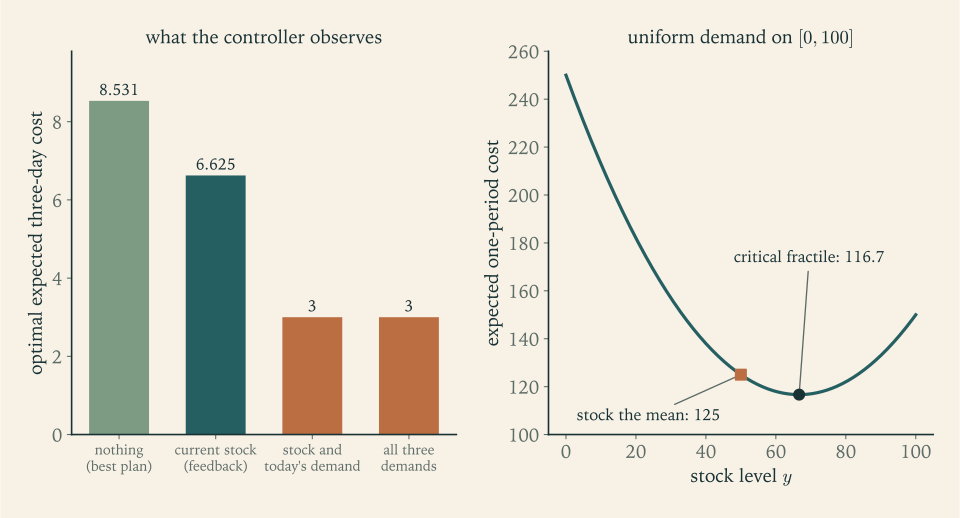
Nothing is observed. The controller must fix a plan. Among plans that respect the shelf capacity on every demand path the best is \((u_0,u_1,u_2)=(1,1,0)\) , with expected cost \(\tfrac{273}{32}\approx8.531\) .
The stock is observed each morning. This is the model of Chapter 2, with optimal cost \(\tfrac{53}{8}=6.625\) .
The stock and the coming day’s demand are observed each morning. The recursion now has the expectation outside the minimum, \(\hat J_k(x)=E\big[\min_u\{g(x,u,w)+\hat J_{k+1}(\max\{0,x+u-w\})\}\big]\) . From an empty shelf the manager orders exactly the demand, pays for it, and ends the day with an empty shelf again: no holding, no shortage. The cost of a day is its demand, with mean \(1\) , so \(\hat J_0(0)=3\) .
All three demands are known at the outset. The same policy, ordering each day’s demand that morning, is still available and still incurs only the unavoidable purchase cost. The expected cost is again \(3\) .
So feedback on the stock is worth \(8.531-6.625=1.906\) ; knowing each day’s demand that morning is worth a further \(3.625\) ; and knowing later demands in advance is worth nothing more, because with instant delivery there is nothing to be done about tomorrow’s demand today. The last step illustrates the equality case of Proposition 6.3.
Common mistake. Reporting the cost of an anticipative rule as if it were achievable. The rule “order today’s demand” costs \(3\) in the shop, less than half of the optimal \(6.625\) . That does not show that dynamic programming failed to find the best policy. It shows what a perfect one-day forecast would be worth. In a simulation, the error appears as a control computed from a disturbance sample that is drawn, in the code, before the control. The test is the one in Definition 6.1: write down the history \(h_k\) and check that the control is a function of it.
Bounds of this kind are useful even when the information is unobtainable. The cost with full knowledge of the disturbances is computed by solving one deterministic problem per disturbance path, which is often easy, and it is a lower bound on the optimal cost of the real problem. If a proposed policy comes close to the bound, the policy is nearly optimal, and no dynamic program need be solved to know it.
6.4 The one case where uncertainty can be ignored
Add a disturbance to the linear-quadratic regulator of Theorem 3.5:
where the \(w_k\) are independent random vectors with mean zero and covariance matrix \(W\) , independent of the states and controls, and the state is observed exactly. The cost is the expected value of the same quadratic expression as before.
Theorem 6.4 (certainty equivalence for the linear-quadratic problem). Let \(Q\succeq0\) , \(Q_N\succeq0\) , \(R\succ0\) , and let \(K_k\) and \(L_k\) be the matrices of Theorem 3.5. For the system with disturbances as above, the optimal policy is \(\mu_k^\star(x)=-L_kx\) , the same as for the deterministic problem, and the optimal cost-to-go is
Proof. By backward induction, with the claim at stage \(k+1\) written \(J_{k+1}(x)=x^{\top}Kx+q\) , where \(K=K_{k+1}\) and \(q\) is the constant. For fixed \(x\) and \(u\) put \(z=Ax+Bu\) . Then
because \(E[w_k]=0\) and \(E[w_k^{\top}Kw_k]=\sum_{i,j}K_{ij}E[w_{k,i}w_{k,j}]=\operatorname{tr}(KW)\) . So the quantity to be minimized over \(u\) is the deterministic one of Theorem 3.5 plus the constant \(\operatorname{tr}(KW)+q\) , which does not involve \(u\) . The minimizer and the quadratic part are therefore those of Theorem 3.5, and the constant accumulates as stated.
The disturbance raises the cost and leaves the policy untouched. A controller may therefore replace each future disturbance by its mean, solve the resulting deterministic problem, and apply the first control; when the state is next observed, repeat. This procedure is called certainty-equivalent control, and the theorem says that for linear dynamics, quadratic cost, additive disturbances, no control constraints, and exact state observation it is optimal. Each of those five conditions is needed.
The reason is visible in the proof. A quadratic function of \(z+w\) splits into a part depending on \(z\) alone and a part depending on \(w\) alone, plus a cross term that vanishes in expectation. Only the mean and covariance of the disturbance enter, and the covariance enters the cost only. No other common cost has this property.
Example 6.3: The scalar regulator with noise
Take Example 3.4, \(x_{k+1}=x_k+u_k+w_k\) with \(N=4\) , and let the \(w_k\) have mean \(0\) and variance \(\sigma^{2}=\tfrac14\) . The gains are unchanged: \(L_0=\tfrac{21}{34}\) , \(L_1=\tfrac{8}{13}\) , \(L_2=\tfrac35\) , \(L_3=\tfrac12\) . From \(x_0=1\) the optimal expected cost is
The check is a direct computation of second moments: under \(u_k=-L_kx_k\) , \(E[x_{k+1}^{2}]=(1-L_k)^{2}E[x_k^{2}]+\sigma^{2}\) , and summing \((1+L_k^{2})E[x_k^{2}]\) over the stages, plus \(E[x_4^{2}]\) , gives \(\tfrac{26931}{8840}\approx3.046\) .
For comparison, the “deadbeat” policy \(u_k=-x_k\) , which cancels the state completely at every stage, costs \(3.75\) . It over-controls: each disturbance is removed in one step at full price, where the optimal policy removes about \(60\) percent per step.
6.5 Where the average misleads
Outside the linear-quadratic family, replacing a random quantity by its mean changes the decision. The cleanest illustration is a one-period inventory problem, which also yields a formula used constantly in practice.
A quantity \(y\) is stocked at unit cost \(c\) before a random demand \(w\) with finite mean and distribution function \(F(y)=P(w\le y)\) is seen. Leftover stock costs \(h\) per unit and unmet demand \(b\) per unit, with \(b\) greater than \(c\) and \(c+h\) positive. The holding cost \(h\) may be negative, as when leftover stock has a salvage value, provided \(c+h\) is positive. The expected cost is
Theorem 6.5 (critical fractile). \(G\) is convex, and it is minimized at the smallest \(y\) for which
Proof. Since \(\max\{0,y-w\}=(y-w)+\max\{0,w-y\}\) ,
For each fixed \(w\) the function \(\max\{0,w-y\}\) is convex in \(y\) , an expectation of convex functions is convex, and \(b+h=(b-c)+(c+h)\) is positive; so \(G\) is the sum of a linear function and a positive multiple of a convex one, and is convex. The right-hand derivative of \(\max\{0,w-y\}\) in \(y\) is \(-1\) if \(w\) exceeds \(y\) and \(0\) otherwise. Taking expectations, the right-hand derivative of \(G\) is
A convex function of one variable is minimized at the smallest point where its right-hand derivative is nonnegative, and \(G'_{+}(y)\ge0\) is the stated inequality. Such a point exists, and the set of such points is bounded below, because \(F(y)\to1\) as \(y\to+\infty\) , \(F(y)\to0\) as \(y\to-\infty\) , and the ratio \(\tfrac{b-c}{b+h}\) lies strictly between \(0\) and \(1\) .
The ratio \(\tfrac{b-c}{b+h}\) compares the cost of having one unit too few, \(b-c\) , with the cost of having one too many, \(c+h\) . The optimal stock is a quantile of the demand distribution, and which quantile depends on the costs. It is the mean only by coincidence.
Example 6.4: Stocking the mean
Let demand be uniformly distributed on \([0,100]\) , with \(c=1\) , \(h=1\) , \(b=5\) . The critical ratio is \(\tfrac{4}{6}=\tfrac23\) , so the optimal stock is \(y^\star=\tfrac{200}{3}\approx66.7\) . Certainty-equivalent reasoning replaces demand by its mean and stocks \(50\) .
For this distribution \(E[\max\{0,y-w\}]=\tfrac{y^{2}}{200}\) and \(E[\max\{0,w-y\}]=\tfrac{(100-y)^{2}}{200}\) , so
Stocking the mean costs \(8.33\) more, about \(7\) percent. With a shortage cost of \(b=20\) the optimal stock rises to \(90.5\) and the certainty-equivalent stock stays at \(50\) .
For the shop of Example 1.1 the ratio is again \(\tfrac23\) , and \(F(0)=\tfrac14\) , \(F(1)=\tfrac34\) : the smallest \(y\) with \(F(y)\ge\tfrac23\) is \(1\) , in agreement with the last-day rule of Example 2.1. On that day the certainty-equivalent stock, the mean demand \(1\) , happens to be right. On the earlier days it is not: certainty equivalence still says “order up to one”, which is the myopic policy of Example 2.2 and costs \(7\) against \(6.625\) .
6.6 Structure that survives uncertainty: base-stock policies
The critical fractile describes one period. Over several periods the optimal ordering rule keeps a simple form, which can be proved without computing anything. Let stock be a real number that may be negative, a negative value being a backlog of unmet demand to be filled later:
with independent nonnegative demands \(w_k\) taking finitely many values, stage cost \(cu_k+h\max\{0,x_{k+1}\}+b\max\{0,-x_{k+1}\}\) , zero terminal cost, and constants satisfying \(h\ge0\) , \(b\) greater than \(c\ge0\) , and \(c+h\) positive.
Theorem 6.6 (base-stock policies). In this model each \(J_k\) is convex, and there are numbers \(S_0,\dots,S_{N-1}\) such that the policy
is optimal: if the stock is below \(S_k\) , order up to \(S_k\) ; otherwise order nothing.
Proof. Write \(y=x+u\) for the stock after ordering and \(H(y)=E[h\max\{0,y-w\}+b\max\{0,w-y\}]\) . The recursion becomes
Suppose \(J_{k+1}\) is convex and nonnegative, as \(J_N=0\) is. Then \(G_k\) is convex, being a sum of convex functions and an average of translates of a convex function. Since \(J_{k+1}\ge0\) , \(G_k(y)\ge cy+h\,E[\max\{0,y-w\}]\) , which tends to \(+\infty\) as \(y\to+\infty\) because \(c+h\) is positive, and \(G_k(y)\ge cy+b\,(E[w]-y)\) , which tends to \(+\infty\) as \(y\to-\infty\) because \(b\) exceeds \(c\) . A convex function that tends to \(+\infty\) in both directions has a minimizer; call it \(S_k\) . Being convex, \(G_k\) is nondecreasing to the right of \(S_k\) , so the minimum over \(y\ge x\) is attained at \(y=S_k\) when \(x\le S_k\) and at \(y=x\) otherwise. That is the base-stock rule.
It remains to see that \(J_k\) is convex and nonnegative. Nonnegativity holds because all costs are. For convexity, let \(m(x)=\min_{y\ge x}G_k(y)\) . Given \(x_1,x_2\) with minimizers \(y_1\ge x_1\) and \(y_2\ge x_2\) , and \(\lambda\in[0,1]\) , the point \(\lambda y_1+(1-\lambda)y_2\) is at least \(\lambda x_1+(1-\lambda)x_2\) , so \(m(\lambda x_1+(1-\lambda)x_2)\le G_k(\lambda y_1+(1-\lambda)y_2)\le\lambda m(x_1)+(1-\lambda)m(x_2)\) . So \(m\) is convex, and \(J_k=m-cx\) is convex.
The facts about convex functions used here, that sums and averages preserve convexity and that a convex function of one variable is monotone on each side of a minimizer, are developed in Continuous Optimization (math.continuous-optimization.convex-sets-functions). The theorem needs the ordering cost to be linear. With a fixed charge for placing any order the functions \(J_k\)
are no longer convex and the optimal rule changes form: it becomes worthwhile to wait until the stock is well below the target before ordering.
Example 6.5: Base-stock levels for three days
Use the costs and demand distribution of the shop, \(c=1\) , \(h=1\) , \(b=5\) , demand \(0,1,2\) with probabilities \(\tfrac14,\tfrac12,\tfrac14\) , but with backlogging and no shelf capacity, for \(N=3\) .
At the last stage \(G_2(y)=y+H(y)\) , the one-period cost: \(G_2(0)=5\) , \(G_2(1)=\tfrac52\) , \(G_2(2)=3\) , \(G_2(3)=5\) . The minimizer is \(S_2=1\) , the critical fractile again, and \(J_2(x)=G_2(\max\{x,1\})-x\) .
At stage \(1\) , adding \(E[J_2(y-w)]\) : \(G_1(0)=\tfrac{17}{2}\) , \(G_1(1)=5\) , \(G_1(2)=\tfrac{37}{8}\) , \(G_1(3)=\tfrac{51}{8}\) , so \(S_1=2\) . At stage \(0\) : \(G_0(1)=\tfrac{57}{8}\) , \(G_0(2)=\tfrac{53}{8}\) , \(G_0(3)=\tfrac{129}{16}\) , so \(S_0=2\) .
The base-stock levels are \(2,2,1\) . The policy found by table in Example 2.1 for the lost-sales shop has the same form, and the end-of-horizon effect seen there is the drop in the level at the last stage. For the backlogging model Theorem 6.6 says that this form is forced: a computed table that showed an order from stock \(1\) and none from stock \(0\) at some stage would have to contain an arithmetic error.
A structural theorem of this kind changes the computation as well as the understanding. In place of one control per state and stage, the policy is described by \(N\) numbers, and each is found by minimizing a convex function of one variable.
Throughout this chapter the state was observed exactly, and that was one of the five conditions in Theorem 6.4. Chapter 7 removes it. The controller will see only a noisy signal of the state, and the first task will be to find out what, in that situation, the state of the problem is.
Exercises
-
Define the classes of history-dependent randomized, deterministic Markov, and open-loop policies, state the inclusions among them, and say which class Theorem 6.2 shows to be sufficient and under what assumption on the disturbances.
Hint
Order the classes by how much of the history \(h_k\) a rule may use and whether it may randomize: open-loop rules use only \(x_0\) and \(k\) ; deterministic Markov rules use \(x_k\) ; history-dependent rules use all of \(h_k\) ; randomized rules draw the control from a distribution. Theorem 6.2 says deterministic Markov policies achieve the optimum, provided the disturbance distribution at stage \(k\) depends only on \(x_k\) and \(u_k\) , which is the state property.
-
One of two actions must be chosen before the state of the world is known. Action A costs \(2\) in the first state and \(10\) in the second; action B costs \(5\) in either. The first state has probability \(0.7\) . Find the best action, its expected cost, the expected cost with perfect information, and the value of perfect information.
Solution
Without information, each action is judged by its expected cost. Action A: \(0.7\cdot2+0.3\cdot10=4.4\) . Action B: \(5\) . The best action is A, with expected cost \(4.4\) .
With perfect information the action is chosen after the state is revealed. In the first state A is better, at cost \(2\) ; in the second B is better, at cost \(5\) . The expected cost is \(0.7\cdot2+0.3\cdot5=2.9\) .
The value of perfect information is the difference, \(4.4-2.9=1.5\) . It is positive because the best action differs between the two states, which by Proposition 6.3 is exactly the condition for strict inequality. All of it comes from the second state: there the informed decision maker pays \(5\) where the uninformed one pays \(10\) , a saving of \(5\) with probability \(0.3\) .
-
In the setting of Proposition 6.3, show that the value of perfect information is zero when \(c(u,w)=a(u)+d(w)\) for some functions \(a\) and \(d\) , and interpret the result.
Hint
If \(c(u,w)=a(u)+d(w)\) then \(\min_uc(u,w)=\min_ua(u)+d(w)\) for every \(w\) , and the same control minimizes for every \(w\) . Compute both sides of Proposition 6.3. The interpretation: when the disturbance affects the cost but not the comparison between controls, knowing it in advance changes no decision and is worth nothing.
-
For the shop in which the day’s demand is seen before ordering, compute the last-day cost \(\hat J_2(x)\) for \(x=0,1,2\) , and explain why it is larger from a full shelf than from a shelf holding one unit.
Answer
Seeing the demand first, the manager orders \(\max\{0,w-x\}\) . From \(x=0\) the cost is \(w\) : \(\hat J_2(0)=1\) . From \(x=1\) : demand \(0\) leaves one unit, cost \(1\) ; demand \(1\) costs \(0\) ; demand \(2\) needs one unit ordered, cost \(1\) ; so \(\hat J_2(1)=\tfrac14+\tfrac14=\tfrac12\) . From \(x=2\) nothing is ordered and the leftover is \(2,1,0\) : \(\hat J_2(2)=\tfrac14\cdot2+\tfrac12\cdot1=1\) . A full shelf is worse than one unit because with perfect knowledge of demand stock is never needed as insurance, and holding it costs money.
-
For the scalar regulator of Example 6.3 with \(N=2\) , terminal weight \(1\) , noise variance \(\sigma^{2}=1\) , and \(x_0=0\) , compute the optimal expected cost from Theorem 6.4, and compute the expected cost of the best open-loop plan. What is feedback worth here?
Solution
With feedback. By Theorem 6.4 the optimal cost from \(x_0=0\) is \(x_0^{2}K_0+\sigma^{2}(K_1+K_2)\) . From Example 3.4 with a two-stage horizon, \(K_2=1\) and \(K_1=\tfrac32\) , so the cost is \(K_1+K_2=\tfrac32+1=\tfrac52\) .
Open loop. With controls fixed in advance, \(x_1=u_0+w_0\) and \(x_2=u_0+u_1+w_0+w_1\) , so \(E[x_1^{2}]=u_0^{2}+1\) and \(E[x_2^{2}]=(u_0+u_1)^{2}+2\) . The expected cost is
\[ 0+u_0^{2}+\big(u_0^{2}+1\big)+u_1^{2}+\big((u_0+u_1)^{2}+2\big), \]which is minimized at \(u_0=u_1=0\) with value \(3\) .
Feedback is worth \(3-\tfrac52=\tfrac12\) . The plan can do nothing about disturbances it cannot see, so its best choice is to do nothing at all; the feedback policy waits for \(w_0\) to show itself in \(x_1\) and then removes half of it, at a control cost that is less than the state cost saved.
-
Let \(w\) be a random vector with mean zero and covariance matrix \(W\) , and let \(K\) be a symmetric matrix. Prove that \(E[w^{\top}Kw]=\operatorname{tr}(KW)\) , and find the corresponding formula when \(w\) has mean \(m\) .
Solution
Write \(w=(w_1,\dots,w_n)\) . Then \(w^{\top}Kw=\sum_{i,j}K_{ij}w_iw_j\) , a finite sum, so by linearity of expectation
\[ E[w^{\top}Kw]=\sum_{i,j}K_{ij}E[w_iw_j]=\sum_{i,j}K_{ij}W_{ij}, \]since \(E[w_iw_j]=W_{ij}\) when the mean is zero. The trace of \(KW\) is \(\sum_i(KW)_{ii}=\sum_i\sum_jK_{ij}W_{ji}\) , and \(W_{ji}=W_{ij}\) because a covariance matrix is symmetric. So \(E[w^{\top}Kw]=\operatorname{tr}(KW)\) .
If \(w\) has mean \(m\) , write \(w=m+v\) with \(v\) of mean zero and covariance \(W\) . Then \(w^{\top}Kw=m^{\top}Km+2m^{\top}Kv+v^{\top}Kv\) , and taking expectations the middle term vanishes: \(E[w^{\top}Kw]=m^{\top}Km+\operatorname{tr}(KW)\) . In the regulator a nonzero mean would shift the deterministic part of the next state and so change the optimal control by a constant, while the covariance would still affect only the cost.
-
Consider the one-stage problem of minimizing \(E[(x_0+\theta u)^{2}]\) over \(u\) , where \(\theta\) is a random gain with mean \(1\) and variance \(\sigma^{2}\) . Find the optimal control, the certainty-equivalent control, and the cost of each, and say which condition of Theorem 6.4 is violated.
Solution
Expand: \(E[(x_0+\theta u)^{2}]=x_0^{2}+2x_0u\,E[\theta]+u^{2}E[\theta^{2}]=x_0^{2}+2x_0u+(1+\sigma^{2})u^{2}\) , since \(E[\theta^{2}]=1+\sigma^{2}\) . This is a convex quadratic in \(u\) with minimizer \(u^\star=-\dfrac{x_0}{1+\sigma^{2}}\) and minimum value \(x_0^{2}-\dfrac{x_0^{2}}{1+\sigma^{2}}=\dfrac{\sigma^{2}}{1+\sigma^{2}}x_0^{2}\) .
Certainty equivalence replaces \(\theta\) by its mean \(1\) and minimizes \((x_0+u)^{2}\) , giving \(u=-x_0\) . Its true cost is \(x_0^{2}-2x_0^{2}+(1+\sigma^{2})x_0^{2}=\sigma^{2}x_0^{2}\) , larger than the optimum by the factor \(1+\sigma^{2}\) . With \(\sigma^{2}=1\) the optimal control is half the certainty-equivalent one and costs half as much.
The violated condition is that the disturbance be additive. Here it multiplies the control, so a larger control injects more uncertainty, and the optimal policy is cautious: it gives up some of the correction to avoid some of the noise.
-
A student simulates the shop under the rule “each morning order exactly the number of units that customers will ask for that day”, obtains an average three-day cost close to \(3\) , and concludes that the table of Example 2.1 is not optimal. Identify the error precisely, using Definition 6.1, and say what the number \(3\) does measure.
Solution
The rule chooses \(u_k=w_k\) when the shelf is empty. The demand \(w_k\) is realized after the order in the model of Example 1.1, so it is not part of the history \(h_k=(x_0,u_0,\dots,x_k)\) , and the rule is not a policy in the sense of Definition 6.1: it is anticipative. In the simulation the demand sample was presumably drawn at the top of the loop and then used to compute the order.
The number \(3\) is the optimal cost of a different model, in which the day’s demand is observed before ordering; Example 6.2 computes it. It is a valid lower bound on the cost of any admissible policy in the original model, by the sequential form of Proposition 6.3, and the gap \(6.625-3=3.625\) is the value of a perfect one-day demand forecast. It says nothing against the optimality of the table of Example 2.1 within the class of policies that can actually be implemented.
-
A colleague argues that “tossing a coin between two good orders hedges against demand uncertainty and so lowers the expected cost”. Refute the claim with the step of the proof of Theorem 6.2 that applies, and illustrate it with the Q-factors \(Q_1(0,1)\) and \(Q_1(0,2)\) of Example 2.1.
Hint
The expected cost of a randomized choice at a state is the weighted average of the Q-factors of the controls it mixes, and an average is never below the smallest of them. With \(Q_1(0,1)=\tfrac{19}{4}\) and \(Q_1(0,2)=\tfrac{37}{8}\) , mixing with weight \(\lambda\) on the first gives \(\tfrac{37}{8}+\tfrac{\lambda}{8}\) , minimized at \(\lambda=0\) . Hedging against demand is already inside each Q-factor, which is an expectation over demand.
-
Demand takes the values \(0,1,2,3,4\) with probabilities \(0.1,0.2,0.3,0.25,0.15\) , and \(c=2\) , \(h=1\) , \(b=8\) . Find the optimal stock by Theorem 6.5 and confirm it by computing \(G(2)\) , \(G(3)\) , and \(G(4)\) .
Solution
The critical ratio is \(\dfrac{b-c}{b+h}=\dfrac{8-2}{8+1}=\dfrac23\) . The distribution function is \(F(0)=0.1\) , \(F(1)=0.3\) , \(F(2)=0.6\) , \(F(3)=0.85\) , \(F(4)=1\) . The smallest \(y\) with \(F(y)\ge\tfrac23\) is \(y^\star=3\) .
To confirm, compute \(G(y)=2y+E[\max\{0,y-w\}]+8E[\max\{0,w-y\}]\) . For \(y=2\) : surplus \(0.1\cdot2+0.2\cdot1=0.4\) , shortage \(0.25\cdot1+0.15\cdot2=0.55\) , so \(G(2)=4+0.4+4.4=8.8\) . For \(y=3\) : surplus \(0.1\cdot3+0.2\cdot2+0.3\cdot1=1.0\) , shortage \(0.15\) , so \(G(3)=8.2\) . For \(y=4\) : surplus \(0.4+0.6+0.6+0.25=1.85\) , shortage \(0\) , so \(G(4)=9.85\) .
The minimum is at \(y=3\) . The mean demand is \(2.15\) , so stocking the rounded mean, \(2\) , would cost \(8.8\) , about \(7\) percent more; the high shortage cost pushes the optimal stock above the mean.
-
Demand is exponentially distributed with mean \(10\) , so that \(F(y)=1-e^{-y/10}\) , and \(c=1\) , \(h=1\) , \(b=5\) . Find the optimal stock and compare it with the mean demand.
Answer
The ratio is \(\tfrac23\) , so \(1-e^{-y/10}=\tfrac23\) and \(y^\star=10\log3\approx10.99\) , about \(10\) percent above the mean demand of \(10\) .
-
In Example 6.5 compute \(J_2(x)\) for \(x=0,1,2,3\) from \(J_2(x)=G_2(\max\{x,1\})-x\) , and verify that these four values are consistent with convexity.
Answer
\(J_2(0)=G_2(1)-0=\tfrac52\) , \(J_2(1)=G_2(1)-1=\tfrac32\) , \(J_2(2)=G_2(2)-2=1\) , \(J_2(3)=G_2(3)-3=2\) . The successive differences are \(-1\) , \(-\tfrac12\) , \(+1\) , which increase, as convexity requires.
-
Suppose placing any order costs a fixed amount \(A\) in addition to \(c\) per unit. For the one-period problem with the function \(G_2\) of Example 6.5, for which \(G_2(-1)=9\) , and \(A=3\) , find the optimal decision from each of the stocks \(x=-1,0,1\) , and explain why the rule is not a base-stock rule.
Answer
Not ordering from stock \(x\) costs \(G_2(x)-x\) ; ordering up to \(y\) costs \(3+G_2(y)-x\) , best at \(y=1\) with \(3+\tfrac52=\tfrac{11}{2}\) before subtracting \(x\) . From \(x=-1\) : \(G_2(-1)=9\) exceeds \(\tfrac{11}{2}\) , so order up to \(1\) . From \(x=0\) : \(G_2(0)=5\) is less than \(\tfrac{11}{2}\) , so do not order, although the stock is below \(1\) . From \(x=1\) : do not order. The rule is “order up to \(1\) only when the stock has fallen to \(-1\) or below”: two numbers, a trigger and a target, where a base-stock rule has one.
-
Consider the rule of Example 6.1 that orders up to two units on the last day only if the previous day’s demand was \(2\) . Without enumerating paths, compute how much it loses relative to the optimal policy, using the Q-factors of Example 2.1 and the probability of the event on which the two policies differ.
Solution
The two policies agree on days \(0\) and \(1\) , where both fill the shelf, so they generate the same distribution of the stock on the morning of day \(2\) and the same cost up to then. They differ on day \(2\) only on the event that the demand of day \(1\) was \(2\) .
On that event the shelf, which held \(2\) units after the order of day \(1\) , is empty on the morning of day \(2\) . The optimal policy orders one unit, at expected cost \(Q_2(0,1)=\tfrac52\) ; the rule orders two, at expected cost \(Q_2(0,2)=3\) . The loss on the event is \(\tfrac12\) .
The event has probability \(\tfrac14\) , and day \(2\) is the last day, so nothing further depends on the choice. The expected loss is \(\tfrac14\cdot\tfrac12=\tfrac18\) , in agreement with the enumeration in Example 6.1, where the rule cost \(\tfrac{27}{4}\) against \(\tfrac{53}{8}\) . The calculation shows the general pattern behind Theorem 6.2: a history-dependent rule can differ from the optimal Markov rule only by choosing, on some histories, a control with a larger Q-factor.
-
For the two-state machine of Example 4.1 with \(\alpha=0.9\) , consider the randomized stationary policy that overhauls a worn machine with probability \(q\) and runs it otherwise. Compute its cost from the worn state as a function of \(q\) and show that it is minimized at \(q=1\) .
Solution
Let \(J(1)\) and \(J(2)\) be the costs from the good and worn states. In the worn state the policy pays \(5\) and moves to good with probability \(q\) , and pays \(2\) and stays worn with probability \(1-q\) :
\[ J(2)=q\,\big(5+0.9J(1)\big)+(1-q)\big(2+0.9J(2)\big),\qquad J(1)=0.9\,\big(0.7J(1)+0.3J(2)\big). \]The second equation gives \(J(1)=\tfrac{27}{37}J(2)\) . Substituting, \(J(2)\big[1-0.9(1-q)-0.9q\cdot\tfrac{27}{37}\big]=2+3q\) , and the bracket is \(0.1+0.9q\cdot\tfrac{10}{37}=\tfrac{3.7+9q}{37}\) . Hence
\[ J(2)=\frac{37\,(2+3q)}{3.7+9q}. \]At \(q=0\) this is \(20\) , and at \(q=1\) it is \(\tfrac{185}{12.7}=14.567\) , the two values of Example 4.1. The derivative has the sign of \(3\,(3.7+9q)-9\,(2+3q)=11.1-18\) , which is negative for every \(q\) . So the cost decreases as \(q\) increases and is smallest at \(q=1\) .
The randomized policies interpolate between the two deterministic ones and none of them is better than the better endpoint, as Theorem 6.2 requires. In the infinite-horizon discounted setting the same conclusion follows from Theorem 4.6.
-
A weather forecast for tomorrow’s inflow is issued each evening before the reservoir release is chosen. Explain how to formulate the problem so that using the forecast is nonanticipative, and what in the formulation would have to change if the forecast were issued only after the release.
Hint
Put the forecast in the state: it is observed before the control, so by the order-of-events rule of Section 1.1 it belongs with the level. The disturbance then generates the inflow from its conditional distribution given the forecast, and the next forecast. If the forecast arrives after the release, it cannot be used for that release; it becomes part of the next stage’s state, where it is useful only if inflows on successive days are dependent.
-
Show that in the model of Theorem 6.4 the best open-loop plan from \(x_0\) is the control sequence of the deterministic problem, and that the cost of feedback over the plan is nonnegative, by comparing the two expected costs for the scalar case \(N=2\) of Exercise 5.
Hint
For a fixed plan the state is \(x_k=\bar x_k+e_k\) , where \(\bar x_k\) follows the deterministic dynamics and \(e_k\) is the accumulated noise, which does not depend on the plan. Expand the quadratic cost: the cross terms vanish in expectation, so the plan-dependent part is the deterministic cost, minimized by the deterministic plan. For the scalar case, compare the \(3\) and \(\tfrac52\) of Exercise 5.
-
For the decision of Exercise 2, find the action that minimizes the worst-case cost, compare it with the action that minimizes the expected cost, and find the probability of the first state at which the expected-cost criterion is indifferent between the two actions.
Answer
Worst cases: A can cost \(10\) , B costs \(5\) ; the worst-case criterion picks B, while the expected-cost criterion picked A. With probability \(p\) for the first state, A has expected cost \(2p+10(1-p)\) , which equals \(5\) at \(p=\tfrac58\) . For \(p\) above \(\tfrac58\) the expected-cost criterion prefers A; below it, B.