A small shop sells one product. Each morning the manager may order more units, which arrive at once; during the day a random number of customers each ask for one unit; unsold units are kept overnight at a cost, and customers who find the shelf empty are lost at a larger cost. The manager wants an ordering rule for the next three days.
Three questions hide in this description. What exactly is being chosen: three order quantities fixed in advance, or a rule that looks at the shelf each morning? What must the manager know each morning in order to decide well: only the stock, or also yesterday’s demand, or last week’s? And how many candidate rules are there, so that we know whether listing them all is a serious option? This chapter answers the three questions. It defines the model that the rest of the book works with, separates plans from policies, and says precisely what it means for a description of the present to be a state.
1.1 The ingredients of a sequential decision problem
Definition 1.1 (finite-horizon model). A finite-horizon stochastic control model with horizon \(N\) consists of, for each stage \(k=0,1,\dots,N-1\) : a set \(S_k\) of states; for each state \(x\in S_k\) a nonempty set \(U_k(x)\) of admissible controls; a set \(D_k\) of disturbances together with a probability distribution \(P_k(\cdot\mid x,u)\) on \(D_k\) for each state \(x\) and admissible control \(u\) ; a system function \(f_k\) giving the next state
and a stage cost \(g_k(x_k,u_k,w_k)\) . There is also a set \(S_N\) of final states and a terminal cost \(g_N(x_N)\) . The disturbance \(w_k\) is drawn from \(P_k(\cdot\mid x_k,u_k)\) ; given \(x_k\) and \(u_k\) it is independent of everything that happened before stage \(k\) .
Until Chapter 3 all the sets are finite, so every expectation in sight is a finite sum and no question of convergence or measurability arises. The definition has one clause that carries far more weight than its length suggests: the distribution of \(w_k\) may depend on the current state and control, and on nothing else from the past. Section 1.3 is devoted to that clause.
The order of events inside a stage is part of the model. At stage \(k\) the decision maker observes \(x_k\) , then chooses \(u_k\in U_k(x_k)\) , and only then is \(w_k\) realized. The control cannot depend on \(w_k\) . A model in which some random quantity is seen before the decision is a different model, obtained by moving that quantity into the state.
Example 1.1: The shop as a model
Let the shelf hold at most \(2\) units, so the stock at the start of day \(k\) is \(x_k\in\{0,1,2\}\) . The order \(u_k\) must satisfy \(x_k+u_k\le 2\) , so \(U_k(x)=\{0,1,\dots,2-x\}\) . Demand \(w_k\) takes the values \(0\) , \(1\) , \(2\) with probabilities \(\tfrac14\) , \(\tfrac12\) , \(\tfrac14\) , independently from day to day and whatever the stock. Unmet demand is lost, so
Each unit ordered costs \(1\) , each unit left on the shelf at the end of the day costs \(1\) to hold, and each unit of unmet demand costs \(5\) :
There is no terminal cost, \(g_N\equiv 0\) , and the horizon is \(N=3\) .
The quantity that matters for a decision is the expected stage cost \(\bar g(x,u)=E[g_k(x,u,w_k)]\) . With \(y=x+u\) units on the shelf after the order arrives, the expected holding cost is \(E[\max\{0,y-w\}]\) and the expected shortage is \(E[\max\{0,w-y\}]\) . For \(y=0\) these are \(0\) and \(1\) ; for \(y=1\) they are \(\tfrac14\) and \(\tfrac14\) ; for \(y=2\) they are \(1\) and \(0\) . Therefore
| State \(x\) | Control \(u\) | Expected stage cost \(\bar g(x,u)\) |
|---|---|---|
| \(0\) | \(0\) | \(0+0+5\cdot 1=5\) |
| \(0\) | \(1\) | \(1+\tfrac14+5\cdot\tfrac14=\tfrac52\) |
| \(0\) | \(2\) | \(2+1+0=3\) |
| \(1\) | \(0\) | \(0+\tfrac14+\tfrac54=\tfrac32\) |
| \(1\) | \(1\) | \(1+1+0=2\) |
| \(2\) | \(0\) | \(0+1+0=1\) |
Looking only at today, the best order from an empty shelf is one unit, at expected cost \(\tfrac52\) . Whether that is the best order when two more days follow is exactly the kind of question the model exists to answer, and Chapter 2 will show that the answer is no.
1.2 Plans and policies
There are two ways to say what the manager will do. An open-loop plan fixes the controls \(u_0,u_1,\dots,u_{N-1}\) at the outset. A closed-loop policy fixes rules.
Definition 1.2 (policy, cost of a policy, optimal cost). A policy is a sequence \(\pi=(\mu_0,\mu_1,\dots,\mu_{N-1})\) of functions with \(\mu_k(x)\in U_k(x)\) for every \(x\in S_k\) . Under \(\pi\) , starting from \(x_0\) , the states and costs are the random variables generated by \(x_{k+1}=f_k(x_k,\mu_k(x_k),w_k)\) . The expected cost of \(\pi\) from \(x_0\) is
The optimal cost is \(J^\star(x_0)=\min_\pi J_\pi(x_0)\) , and a policy \(\pi^\star\) is optimal if \(J_{\pi^\star}(x_0)=J^\star(x_0)\) for every initial state \(x_0\in S_0\) .
A policy as defined here looks only at the current state. That restriction is harmless under Definition 1.1, though it takes a theorem to say so; Chapter 6 proves that rules which consult the entire history, or toss coins, cannot do better. The minimum in the definition of \(J^\star\) exists because, with finite sets, there are finitely many policies. The definition of an optimal policy is stronger than it had to be: it asks for one policy that is best from every starting state at once. That such a policy exists is the first theorem of Chapter 2.
A policy is a much larger object than a plan. A plan is one control per stage; a policy is one control per stage per state. The extra size is what lets it react.
Example 1.2: A plan against a policy over two days
Take the shop of Example 1.1 with horizon \(N=2\) and an empty shelf, \(x_0=0\) .
An open-loop plan. Order one unit each morning, \(u_0=u_1=1\) . Day 0 costs \(\bar g(0,1)=\tfrac52\) in expectation. The stock next morning is \(x_1=\max\{0,1-w_0\}\) , which is \(1\) with probability \(\tfrac14\) and \(0\) with probability \(\tfrac34\) . On day 1 the plan orders one unit regardless, costing \(\bar g(1,1)=2\) or \(\bar g(0,1)=\tfrac52\) . The expected total is
Listing all six plans that respect the shelf capacity on every demand path gives the following costs.
| Plan \((u_0,u_1)\) | \((0,0)\) | \((0,1)\) | \((0,2)\) | \((1,0)\) | \((1,1)\) | \((2,0)\) |
|---|---|---|---|---|---|---|
| Expected cost | \(10\) | \(\tfrac{15}{2}\) | \(8\) | \(\tfrac{53}{8}\) | \(\tfrac{39}{8}\) | \(\tfrac{21}{4}\) |
So the best open-loop plan costs \(\tfrac{39}{8}=4.875\) .
A policy. Order up to one unit: \(\mu_k(0)=1\) and \(\mu_k(1)=\mu_k(2)=0\) . Day 0 is as before. On day 1 the policy orders only if the shelf is empty, costing \(\bar g(1,0)=\tfrac32\) or \(\bar g(0,1)=\tfrac52\) :
This is \(\tfrac18\) less than the best plan, and the whole saving comes from the one situation, probability \(\tfrac14\) , in which the plan orders a unit that the policy can see is not needed.
A better policy. Order two units on day 0, then order up to one on day 1. Day 0 costs \(\bar g(0,2)=3\) ; the next stock is \(2\) , \(1\) , or \(0\) with probabilities \(\tfrac14,\tfrac12,\tfrac14\) , and day 1 costs \(1\) , \(\tfrac32\) , or \(\tfrac52\) accordingly:
The three numbers \(\tfrac{39}{8}\) , \(\tfrac{38}{8}\) , \(\tfrac{37}{8}\) measure, in order, what can be done without feedback, with a naive feedback rule, and with a feedback rule that also thinks ahead.
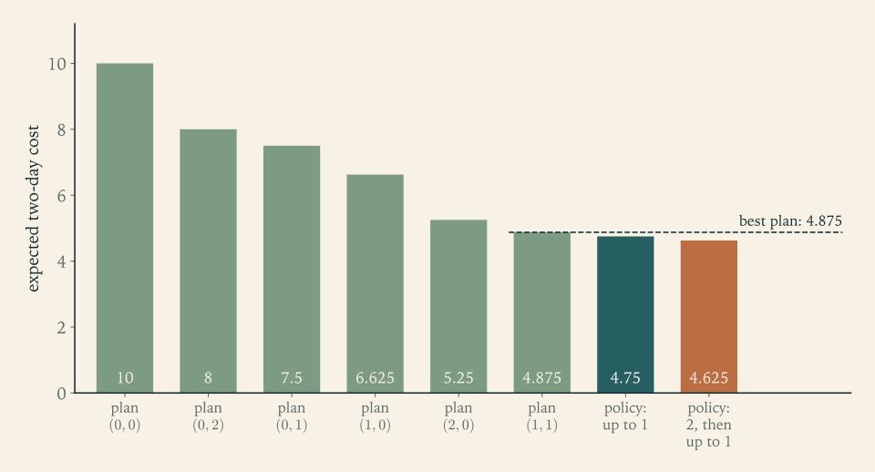
Feedback earns its keep only because the future is uncertain. When nothing is random the two notions coincide.
Proposition 1.3 (no disturbance, no advantage to feedback). Suppose each \(D_k\) has a single element, so that \(x_{k+1}=f_k(x_k,u_k)\) . Then for every initial state \(x_0\) the minimum cost over open-loop plans that are admissible from \(x_0\) equals the minimum cost over policies.
Proof. Fix \(x_0\) . Given a policy \(\pi\) , the recursion \(x_{k+1}=f_k(x_k,\mu_k(x_k))\) produces one definite trajectory, and the controls \(u_k=\mu_k(x_k)\) along it form an admissible open-loop plan that produces the same trajectory and therefore the same cost. Conversely, given an admissible plan \((u_0,\dots,u_{N-1})\) with trajectory \((x_0,\dots,x_N)\) , define a policy by \(\mu_k(x_k)=u_k\) at the trajectory’s state and arbitrarily elsewhere; started from \(x_0\) it reproduces the plan. So the two sets of achievable costs from \(x_0\) are equal, and so are their minima.
The proposition does not make policies useless in deterministic problems. An optimal policy answers the question for every starting state and remains correct if the system is knocked off its planned trajectory, while a plan is tied to one starting state. Chapter 3 computes deterministic optimal policies for exactly that reason.
1.3 What a state has to do
The word state has been used as if its meaning were obvious. It is not, and most modelling errors in this subject are errors about the state.
Definition 1.4 (the state property). A variable \(x_k\) has the state property for a sequential decision problem if, at every stage \(k\) , the following depend on the past only through the current value of \(x_k\) : the set of admissible controls; the conditional distribution of the disturbance \(w_k\) given the whole past and the current control; the next value \(x_{k+1}\) , through \(x_k\) , \(u_k\) , and \(w_k\) ; and the cost incurred at stage \(k\) .
Definition 1.1 builds the state property in. The point of stating it separately is that a real problem does not arrive with its state labelled. One starts with physical variables, and has to check whether they have the state property. The test is a single question: holding the proposed state and the proposed control fixed, can two different pasts lead to different futures or different costs? If they can, the proposed state is too small.
The state property is what makes the future of a controlled system a Markov chain once the policy is fixed.
Lemma 1.5 (a policy turns the model into a Markov chain). Under Definition 1.1 and a policy \(\pi\) , the state sequence satisfies
whenever the conditioning event has positive probability. Consequently, for every stage \(k\) and state \(i\) , the conditional expectation of the remaining cost \(g_N(x_N)+\sum_{m=k}^{N-1}g_m(x_m,\mu_m(x_m),w_m)\) , given \(x_k=i\) and any past, is a function of \(k\) and \(i\) alone.
Proof. Given \(x_k=i\) the control is \(\mu_k(i)\) , and by Definition 1.1 the disturbance \(w_k\) then has distribution \(P_k(\cdot\mid i,\mu_k(i))\) independently of the earlier history. Since \(x_{k+1}=f_k(i,\mu_k(i),w_k)\) , the first claim follows by adding the probabilities of the disturbances that lead to \(j\) .
For the second claim argue backward. At \(k=N\) the remaining cost is \(g_N(x_N)\) , a function of \(x_N\) . Suppose the claim holds at stage \(k+1\) , with the conditional expectation there equal to \(c_{k+1}(x_{k+1})\) . Condition first on \(x_k=i\) , the past, and \(w_k\) : the stage cost is \(g_k(i,\mu_k(i),w_k)\) and the expected remainder is \(c_{k+1}(f_k(i,\mu_k(i),w_k))\) . Averaging over \(w_k\) , whose conditional distribution depends only on \(i\) , gives a quantity \(c_k(i)\) that does not involve the past.
In the language of Stochastic Processes, a fixed policy produces a time-inhomogeneous Markov chain with one-step transition probabilities \(p^k_{ij}(\mu_k(i))\)
(math.stochastic-processes.markov-chain-transition). That course studies what such a chain does. This one studies how to choose the policy, which is to say how to choose the chain. The numbers \(p_{ij}(u)\)
are an alternative way to specify a model: instead of a system function and a disturbance distribution, give the probability of moving from \(i\)
to \(j\)
under control \(u\)
directly. From Chapter 4 onward that is the form used. For the shop, the control \(u=2\)
in state \(0\)
has \(p_{02}(2)=\tfrac14\)
, \(p_{01}(2)=\tfrac12\)
, and \(p_{00}(2)=\tfrac14\)
.
When a natural variable fails the test, the remedy is to enlarge it.
Example 1.3: A start-up cost breaks the state property
A machine can make the shop’s product at a cost of \(1\) per unit, but if it was idle yesterday it must be started today at an extra cost of \(3\) . Alternatively a unit can be bought outside for \(3\) . Today the shelf is empty and exactly one unit is needed. Is the stock level a state?
Apply the test with \(x_k=0\) . If the machine ran yesterday, making the unit costs \(1\) and buying costs \(3\) ; the best action is to make. If the machine was idle yesterday, making costs \(3+1=4\) and buying costs \(3\) ; the best action is to buy. The same stock level and the same proposed action, to make one unit, give a cost of \(1\) after one past and \(4\) after another. The stock level fails the test, and no rule that looks only at the stock can be right in both situations.
The repair is to carry yesterday’s action along. Let \(m_{k}\in\{\text{idle},\text{running}\}\) record whether the machine ran on day \(k-1\) , and take the pair \(z_k=(x_k,m_k)\) as the state. Its second component updates deterministically, since \(m_{k+1}\) records what was done on day \(k\) , and the cost of day \(k\) is now a function of \(z_k\) and \(u_k\) . With three stock levels the state set grows from \(3\) elements to \(6\) .
Example 1.4: Demand that remembers
Suppose demand in the shop is \(1\) on a quiet day and \(2\) on a busy day, that a quiet day is followed by a quiet day with probability \(0.8\) , and that a busy day is followed by a busy day with probability \(0.6\) . The shelf is empty and there is one day to go, with the costs of Example 1.1.
If yesterday was quiet, ordering one unit costs \(1\) plus an expected shortage cost \(5\cdot 0.2=1\) , total \(2\) ; ordering two costs \(2\) plus an expected holding cost \(1\cdot 0.8\) , total \(2.8\) . The better order is \(1\) . If yesterday was busy, ordering one unit costs \(1+5\cdot 0.6=4\) and ordering two costs \(2+1\cdot 0.4=2.4\) . The better order is \(2\) .
Again the stock level fails the test: the distribution of today’s disturbance depends on yesterday’s disturbance. The pair \((x_k,w_{k-1})\) has the state property, because given yesterday’s demand the distribution of today’s demand is known and nothing earlier adds information. The manager must be able to see yesterday’s demand for this to be a usable state; if only sales are recorded and a stock-out hides the true demand, the difficulty is of a different kind, and it is the subject of Chapter 7.
The two examples are instances of general recipes, all of which enlarge the state by exactly the part of the past that still matters.
Delays. If an order placed on day \(k\) arrives on day \(k+1\) , the future depends on the stock and on the order in transit; the state is \((x_k,u_{k-1})\) . A delay of \(d\) stages needs the last \(d\) controls.
Correlated disturbances. If \(w_k\) depends on \(w_{k-1}\) , as in Example 1.4, and \(w_{k-1}\) has been observed, append it. If \(w_k=\rho w_{k-1}+\xi_k\) with independent \(\xi_k\) , the pair \((x_k,w_{k-1})\) is a state and \(\xi_k\) plays the part of the disturbance.
Costs and constraints with memory. If the cost or the admissible set depends on earlier actions, as in Example 1.3, or on a running total, such as a budget of at most \(m\) repairs over the horizon, append the relevant summary: the previous action, or the number of repairs still allowed.
Forecasts. If a forecast \(y_k\) of today’s demand is seen before ordering, then \((x_k,y_k)\) is the state, and the disturbance distribution is the conditional distribution of demand given the forecast.
Time. If the model changes from stage to stage, the pair \((k,x_k)\) is a state of a model that does not.
Common mistake. Treating whatever is physically measured as the state. The stock on the shelf is what the manager sees, but in Examples 1.3 and 1.4 it does not determine the cost of an action or the odds of tomorrow’s demand. The opposite error is as costly in practice: carrying variables that do not pass the test’s other half, in that they change neither the future nor the cost. Every component added to the state multiplies the number of states, and Section 1.5 shows what that does to computation. A state should contain everything from the past that affects the future, and nothing else.
1.4 The forms a cost can take
Definition 1.2 minimizes the expected value of a sum of stage costs. Three features of that objective deserve comment, because each is a modelling choice.
The objective is an expectation. A policy is judged by its average cost over the randomness, which is appropriate when the decision is repeated many times or the stakes are small relative to resources. A decision maker who dislikes variability would want a different objective. Some of these can be brought back to the present form: minimizing the expected value of a convex increasing function of the total cost, for instance, can be handled by carrying the accumulated cost in the state. Others cannot, and they fall outside this book.
The objective is additive over stages. Additivity is what will let Chapter 2 split the problem at any stage into a cost already paid and a cost still to come. Several objectives that do not look additive become so after augmentation. To minimize the probability that the final state lies outside a target set \(A\) , take zero stage costs and the terminal cost \(g_N(x)=1\) for \(x\notin A\) and \(0\) for \(x\in A\) . To minimize the expected largest stage cost, carry the running maximum \(m_k\) as a state component and charge \(g_N(x_N,m_N)=m_N\) at the end.
Constraints on the state are part of the model through the sets \(U_k(x)\) , which may exclude any control that could lead to a forbidden state, or through infinite costs, a device that Chapter 3 treats with care. A problem stated with rewards is a problem with costs after a change of sign; maximizing \(E[\sum r_k]\) and minimizing \(E[\sum(-r_k)]\) have the same optimal policies.
When the horizon is long, a unit of cost tomorrow is often worth less than a unit today. A discount factor \(\alpha\in(0,1)\) weights the stage-\(k\) cost by \(\alpha^{k}\) . With a finite horizon this is one more instance of Definition 1.1, with stage cost \(\alpha^{k}g(x,u,w)\) . Its real importance appears when the horizon is infinite, in Chapter 4.
1.5 Why not try every policy?
With finite sets there are finitely many policies, so in principle one could evaluate each and keep the best. The following count shows how quickly that stops being possible, and what the alternative costs.
Example 1.5: Counting policies in the shop
In the shop a policy must pick, at each stage, one of \(3\) controls in state \(0\) , one of \(2\) in state \(1\) , and the only available control in state \(2\) . That is \(3\cdot 2\cdot 1=6\) rules per stage, hence \(6^{3}=216\) policies for the three-day problem. Evaluating one policy means computing an expected cost over the \(3^{3}=27\) demand paths.
Carrying out this enumeration by machine gives a minimum expected cost from \(x_0=0\) of \(\tfrac{53}{8}\) . Exactly two of the \(216\) policies attain it. They agree in ordering two units on day 0 from an empty shelf, in ordering up to two on day 1, and in ordering up to one on day 2; they differ only in what they would do on day 0 from a stock of \(1\) , which is irrelevant when the shelf starts empty.
Now scale the problem up. A model with \(n\) states, \(m\) controls in each, and \(N\) stages has \(m^{nN}\) policies. With \(n=100\) , \(m=10\) , and \(N=20\) that is \(10^{2000}\) . The method of Chapter 2 solves the same problem by examining each triple of stage, state, and control once: \(N\cdot n\cdot m=20{,}000\) expected values, each a sum over at most \(n\) successor states.
The comparison in Example 1.5 is between \(m^{nN}\) and \(Nnm\) : exponential in the size of the problem against linear in each of its dimensions. That gap is the reason dynamic programming exists.
It is not the end of the story, because \(n\) itself is often enormous. A state with \(d\) components, each taking \(q\) values, has \(n=q^{d}\) elements. Ten components with ten values each give \(10^{10}\) states, and a table over them is out of reach. Bellman called this the curse of dimensionality. It explains two habits of the subject: the care taken in Section 1.3 to keep the state small, and the search for problems with special structure, such as the linear-quadratic problems of Chapters 3, 6, and 9, in which the optimal cost has a closed form and no table is needed. Chapter 10 takes up what to do when neither escape is available.
The questions this chapter leaves open set the agenda. How can the best of \(216\) policies be found without listing them, and why is ordering two units right on day 0 when one unit is cheaper today? Chapter 2 answers with the backward recursion. What changes when nothing is random? Chapter 3. And what replaces the table when the horizon has no end? Chapters 4 and 5.
Exercises
-
A machine is either working or broken at the start of each week. A working machine earns a profit of \(10\) during the week and breaks by the end of it with probability \(0.2\) ; a broken machine earns nothing and can be repaired at a cost of \(4\) , which makes it work for the coming week, or left broken. Write this as a model in the sense of Definition 1.1 with costs equal to negative profits: give the state set, the admissible controls in each state, a disturbance with its distribution, the system function, and the stage cost.
Answer
States: \(S_k=\{\text{working},\text{broken}\}\) . Controls: \(U_k(\text{working})=\{\text{run}\}\) and \(U_k(\text{broken})=\{\text{repair},\text{leave}\}\) . Disturbance: \(w_k\in\{\text{survive},\text{fail}\}\) with \(P(\text{fail})=0.2\) when the machine runs during the week; when it is left broken the disturbance has no effect. System function: a machine that runs (because it was working, or was repaired) is working next week if \(w_k\) is “survive” and broken if “fail”; a machine left broken stays broken. Stage cost: \(-10\) for a working machine, \(4-10=-6\) for a repaired one, \(0\) for a machine left broken.
-
In the shop of Example 1.1 suppose demand is instead \(0\) , \(1\) , or \(2\) with probabilities \(\tfrac12\) , \(\tfrac14\) , \(\tfrac14\) . Recompute the expected holding and shortage quantities for \(y=0,1,2\) units on the shelf, and find the order from an empty shelf that minimizes the expected cost of a single day.
Answer
Expected holding and shortage: for \(y=0\) they are \(0\) and \(\tfrac34\) ; for \(y=1\) they are \(\tfrac12\) and \(\tfrac14\) ; for \(y=2\) they are \(\tfrac54\) and \(0\) . From an empty shelf the one-day expected costs are \(5\cdot\tfrac34=\tfrac{15}{4}\) for \(u=0\) , \(1+\tfrac12+\tfrac54=\tfrac{11}{4}\) for \(u=1\) , and \(2+\tfrac54=\tfrac{13}{4}\) for \(u=2\) . Order one unit.
-
For the shop of Example 1.1 with horizon \(N=2\) and \(x_0=0\) , compute the expected cost of the policy “order up to two units every morning” by the method of Example 1.2, and compare it with the three costs found there.
Solution
Under “order up to two” the shelf holds \(2\) units after every morning’s order. On day 0, starting from \(x_0=0\) , the order is \(u_0=2\) and the expected cost is \(\bar g(0,2)=3\) . The next stock is \(x_1=2-w_0\) , equal to \(2\) , \(1\) , \(0\) with probabilities \(\tfrac14\) , \(\tfrac12\) , \(\tfrac14\) .
On day 1 the policy orders \(0\) , \(1\) , or \(2\) units from those stocks. The expected day-1 cost is the order cost plus the expected holding cost of \(1\) with two units on the shelf: \(\bar g(2,0)=1\) , \(\bar g(1,1)=2\) , \(\bar g(0,2)=3\) . Hence the expected two-day cost is \(3+\tfrac14\cdot 1+\tfrac12\cdot 2+\tfrac14\cdot 3=5\) .
This is worse than all three costs of Example 1.2, namely \(\tfrac{39}{8}\) , \(\tfrac{19}{4}\) , and \(\tfrac{37}{8}\) . Filling the shelf on the last day pays for stock that will be left over with certainty when demand is at most \(2\) and leftover units have no value.
-
For the shop under the policy “order up to one unit”, write the \(3\times 3\) matrix whose entry in row \(i\) and column \(j\) is the probability of moving from stock \(i\) to stock \(j\) in one day, and verify that each row sums to \(1\) .
Solution
Under “order up to one” the control is \(u=1\) in state \(0\) and \(u=0\) in states \(1\) and \(2\) . From state \(0\) or state \(1\) the shelf holds one unit after the order; it is sold unless demand is \(0\) , so the next stock is \(1\) with probability \(\tfrac14\) and \(0\) with probability \(\tfrac34\) . From state \(2\) nothing is ordered and the next stock is \(2-w\) , equal to \(2\) , \(1\) , \(0\) with probabilities \(\tfrac14\) , \(\tfrac12\) , \(\tfrac14\) . With rows and columns indexed by stock \(0,1,2\) ,
\[ P=\begin{pmatrix}\tfrac34&\tfrac14&0\\ \tfrac34&\tfrac14&0\\ \tfrac14&\tfrac12&\tfrac14\end{pmatrix}. \]Each row sums to \(1\) , as it must, since from every state the chain goes somewhere. Notice that state \(2\) can be left but never re-entered under this policy: column \(2\) is zero in rows \(0\) and \(1\) .
-
Suppose an order placed on the morning of day \(k\) is delivered one day late: it reaches the shelf on the morning of day \(k+1\) , in time for that day’s customers but after that day’s order has been placed. Let \(x_k\) be the stock on the shelf when the order of day \(k\) is placed. Show with the test of Section 1.3 that \(x_k\) no longer has the state property, propose a state that does, and write its system function for lost-sales dynamics.
Solution
Apply the test. Fix the stock \(x_k\) and the order \(u_k\) . If yesterday’s order was \(u_{k-1}=0\) , today’s customers face \(x_k\) units; if it was \(u_{k-1}=2\) , they face \(x_k+2\) . The distribution of the shortage cost and of tomorrow’s stock differ, although \(x_k\) and \(u_k\) are the same. So \(x_k\) fails: the cost and the next value depend on the past through something other than \(x_k\) .
What is missing is the order in transit. Let \(q_k=u_{k-1}\) and take \(z_k=(x_k,q_k)\) as the state. During day \(k\) the shelf holds \(x_k+q_k\) units, so
\[ z_{k+1}=\big(\max\{0,\ x_k+q_k-w_k\},\ u_k\big), \]and the stage cost is \(u_k+\max\{0,x_k+q_k-w_k\}+5\max\{0,w_k-x_k-q_k\}\) , a function of \(z_k\) , \(u_k\) , and \(w_k\) . The capacity constraint becomes a condition on \(x_k+q_k+u_k\) or on \(x_k+q_k\) , depending on what the shelf must hold, and in either case depends only on \(z_k\) and \(u_k\) . Today’s order affects nothing until tomorrow, which is why decisions under delay have to look further ahead.
-
Consider \(x_{k+1}=x_k+u_k+w_k\) for \(k=0,1\) with \(x_0=0\) , controls \(u_k\in\{-1,0,1\}\) , disturbances \(w_k\) equal to \(+1\) or \(-1\) with probability \(\tfrac12\) each, no stage costs, and terminal cost \(x_2^{2}\) . Find the minimum expected cost over open-loop plans and the minimum over policies, and explain the difference in one sentence.
Solution
Open loop. The final state is \(x_2=u_0+u_1+w_0+w_1\) . The disturbances have mean \(0\) and variance \(1\) each and are independent, so \(E[x_2^{2}]=(u_0+u_1)^{2}+2\) . This is smallest when \(u_0+u_1=0\) , for instance \(u_0=u_1=0\) , so the open-loop minimum is \(2\) .
Closed loop. At stage 1 the controller knows \(x_1=u_0+w_0\) . Given \(x_1\) , the expected cost is \(E[(x_1+u_1+w_1)^{2}]=(x_1+u_1)^{2}+1\) . Choose \(u_0=0\) , so that \(x_1=\pm1\) , and then \(u_1=-x_1\) , which is admissible. The expected cost is \(0+1=1\) . No policy does better, since \(E[(x_1+u_1+w_1)^{2}\mid x_1]\ge\operatorname{Var}(w_1)=1\) whatever \(u_1\) is. So the closed-loop minimum is \(1\) .
The policy cancels the first disturbance after seeing it; a plan, fixed before \(w_0\) is drawn, cannot, and must carry both variances to the end.
-
In Example 1.3 suppose the start-up cost is charged only if the machine has been idle for the last two days in a row. What must be added to the stock level to obtain a state, how many values does the new component take, and what is its update rule?
Answer
Add the number of consecutive idle days immediately before today, capped at two: \(m_k\in\{0,1,2\}\) , where \(2\) means “two or more”. Update: \(m_{k+1}=0\) if the machine runs on day \(k\) , and \(m_{k+1}=\min\{m_k+1,2\}\) if it is idle. The start-up cost is charged when the machine runs and \(m_k=2\) . With three stock levels there are \(9\) states.
-
A reservoir receives inflow \(w_k=\rho w_{k-1}+\xi_k\) , where the \(\xi_k\) are independent and \(w_{k-1}\) is measured before the release \(u_k\) is chosen; the level evolves by \(x_{k+1}=x_k-u_k+w_k\) . Give a state with the state property, identify the disturbance of the augmented model, and say what goes wrong if past inflows cannot be measured.
Hint
The level alone fails the test because the distribution of \(w_k\) depends on \(w_{k-1}\) . Try the pair \((x_k,w_{k-1})\) and write both components of its update in terms of \(x_k\) , \(w_{k-1}\) , \(u_k\) , and \(\xi_k\) ; then \(\xi_k\) is the disturbance and it is independent of the past. If past inflows cannot be measured, the second component is not available to the decision maker, and a policy cannot be a function of it; that is a problem of partial observation.
-
A maintenance contract allows at most \(2\) overhauls during a horizon of \(N=10\) weeks, and the machine’s condition takes \(4\) values. Define a state that makes the admissible control set depend only on the current state, and count the number of states.
Solution
The admissible set must say whether an overhaul is still permitted, and that depends on how many have been used, which the machine’s condition does not record. Two histories with the same condition, one with no overhauls so far and one with two, allow different controls. So the condition alone fails the first clause of Definition 1.4.
Take the state \(z_k=(c_k,r_k)\) , where \(c_k\) is the condition and \(r_k\in\{0,1,2\}\) is the number of overhauls still allowed. The control “overhaul” is admissible only when \(r_k\ge 1\) , and it sets \(r_{k+1}=r_k-1\) ; any other control leaves \(r_{k+1}=r_k\) . There are \(4\cdot 3=12\) states at each stage. If the stage is also carried as a state component, to make the model stationary, there are \(12\cdot 10=120\) pairs of stage and state, though many are unreachable: at stage \(0\) only \(r_0=2\) can occur.
-
A student models the shop of Example 1.4 with the stock level alone as the state “because the stock is all that is on the shelf”, and concludes that one unit should be ordered whenever the shelf is empty on the last day. Using the numbers of that example, compute the expected cost of this rule on a day that follows a busy day, compare it with the best available cost, and name the clause of Definition 1.4 that the student’s state violates.
Solution
After a busy day, demand is \(2\) with probability \(0.6\) and \(1\) with probability \(0.4\) . The student’s rule orders one unit, at cost \(1\) , and faces a shortage of one unit with probability \(0.6\) : the expected cost is \(1+5\cdot 0.6=4\) . Ordering two units costs \(2\) plus a holding cost of \(1\) with probability \(0.4\) , a total of \(2.4\) . The student’s rule loses \(1.6\) on every last day that follows a busy day.
The violated clause is the second: the conditional distribution of the disturbance \(w_k\) , given the past, must depend on the past only through the state. Here it depends on \(w_{k-1}\) , which the stock level does not determine. “What is on the shelf” describes the physical system; a state must also carry whatever the decision maker knows that changes the odds of the future. With the state \((x_k,w_{k-1})\) the right rule is available: from an empty shelf order \(1\) after a quiet day and \(2\) after a busy day.
-
A model has \(4\) states, \(3\) admissible controls in every state, and horizon \(N=5\) . Count the policies in the sense of Definition 1.2, count the open-loop plans, and count the expected values that a method examining each stage, state, and control once would compute.
Answer
A policy chooses one of \(3\) controls for each of \(4\) states at each of \(5\) stages: \(3^{20}=3{,}486{,}784{,}401\) policies. There are \(3^{5}=243\) open-loop plans. A method that examines each stage, state, and control once computes \(5\cdot 4\cdot 3=60\) expected values.
-
Express each objective as an expected additive cost in the sense of Definition 1.2, enlarging the state if necessary: (a) maximize the probability that \(x_N\ge a\) ; (b) minimize the expected value of the largest stock level reached during the horizon; (c) minimize \(E[\sum_{k}\alpha^{k}g(x_k,u_k,w_k)]\) for a fixed \(\alpha\in(0,1)\) .
Hint
(a) Use zero stage costs and a terminal cost that is \(-1\) on the target and \(0\) off it; the expected cost is then minus the probability. (b) The largest stock so far is not a function of the current stock; carry it as a second state component \(m_k\) , update it by a maximum, and charge it at the end. (c) No augmentation is needed if the stage cost is allowed to depend on \(k\) ; if you want a stage-independent model, look at Exercise 17.
-
Let \(P\) be the matrix of Exercise 4 and let \(\bar g\) be the column vector of expected one-day costs under the policy “order up to one unit”. Show that the vector of expected two-day costs under that policy is \(\bar g+P\bar g\) , compute it, and check its first entry against Example 1.2.
Solution
Let \(c(i)\) be the expected two-day cost from stock \(i\) . The first day costs \(\bar g(i)\) in expectation. The second day starts from a random stock \(x_1\) with \(P(x_1=j)=P_{ij}\) and costs \(\bar g(j)\) in expectation given \(x_1=j\) , because the second day’s demand is independent of the first day’s. Averaging over \(x_1\) , the second day contributes \(\sum_j P_{ij}\bar g(j)\) , the \(i\) -th entry of \(P\bar g\) . Hence \(c=\bar g+P\bar g\) .
With \(\bar g=\big(\tfrac52,\tfrac32,1\big)\) from the table of Example 1.1 (controls \(1\) , \(0\) , \(0\) ) and \(P\) from Exercise 4,
\[ P\bar g=\Big(\tfrac34\cdot\tfrac52+\tfrac14\cdot\tfrac32,\ \ \tfrac34\cdot\tfrac52+\tfrac14\cdot\tfrac32,\ \ \tfrac14\cdot\tfrac52+\tfrac12\cdot\tfrac32+\tfrac14\cdot 1\Big)=\big(\tfrac94,\tfrac94,\tfrac{13}{8}\big), \]so the two-day costs are \(\big(\tfrac{19}{4},\tfrac{15}{4},\tfrac{21}{8}\big)\) . The first entry is the \(\tfrac{19}{4}\) of Example 1.2. The same computation with more factors gives the \(N\) -day cost \(\bar g+P\bar g+\dots+P^{N-1}\bar g\) of a policy that uses the same rule every day.
-
Prove directly from Definition 1.1 that, under a policy \(\pi\) , the expected cost satisfies \(J_\pi(x_0)=E\big[g_0(x_0,\mu_0(x_0),w_0)+c_1(x_1)\big]\) , where \(c_1(i)\) is the expected cost of stages \(1\) to \(N\) under \(\pi\) given \(x_1=i\) . State where the independence clause of Definition 1.1 is used.
Solution
Write the total cost under \(\pi\) as \(g_0(x_0,\mu_0(x_0),w_0)+R\) , where \(R=g_N(x_N)+\sum_{k=1}^{N-1}g_k(x_k,\mu_k(x_k),w_k)\) is the cost of stages \(1\) to \(N\) . By linearity, \(J_\pi(x_0)=E[g_0(x_0,\mu_0(x_0),w_0)]+E[R]\) .
To evaluate \(E[R]\) , condition on \(w_0\) . Given \(w_0\) the next state is the known value \(x_1=f_0(x_0,\mu_0(x_0),w_0)\) . The remaining disturbances \(w_1,\dots,w_{N-1}\) are then generated stage by stage, each from a distribution \(P_k(\cdot\mid x_k,\mu_k(x_k))\) that depends on the current state alone. This is where the independence clause of Definition 1.1 is used: it guarantees that knowing \(w_0\) in addition to \(x_1\) does not change the distribution of anything that follows. Therefore \(E[R\mid w_0]=c_1(x_1)\) , where \(c_1(i)\) is the expected value of \(R\) when the system is started in state \(i\) at stage \(1\) and \(\pi\) is followed. Taking the expectation over \(w_0\) gives \(E[R]=E[c_1(x_1)]\) , and adding the first-stage cost gives the claim.
-
Consider \(x_{k+1}=x_k+u_k\) with no disturbance, \(x_0=8\) , and the policy \(\mu_k(x)=-x/2\) for \(k=0,1,2\) . Write the open-loop plan that Proposition 1.3 associates with this policy, and say what the plan and the policy each do if the initial state is changed to \(x_0=4\) without recomputing anything.
Answer
The trajectory is \(8,4,2,1\) and the plan is \((u_0,u_1,u_2)=(-4,-2,-1)\) . From \(x_0=4\) the policy produces \(4,2,1,\tfrac12\) with controls \((-2,-1,-\tfrac12)\) , still halving the state at each stage; the old plan produces \(4,0,-2,-3\) , which is no longer what the rule intended.
-
A sales forecast \(y_k\in\{\text{low},\text{high}\}\) is published each morning before the order is placed; given the forecast, demand has a known conditional distribution, and forecasts on different days are independent. Formulate the state, the disturbance, and the system function, and explain why the forecast is part of the state while demand is not.
Hint
Recall the order of events: whatever is seen before the control is chosen belongs to the state, and whatever is realized afterwards is a disturbance. The state is \((x_k,y_k)\) . The disturbance must generate both today’s demand, drawn from its conditional distribution given \(y_k\) , and tomorrow’s forecast \(y_{k+1}\) .
-
Show that a model whose sets, system functions, and costs vary with the stage \(k\) can be rewritten as a model in which they do not, by taking \((k,x_k)\) as the state. Write the new state set, admissible controls, system function, and stage cost.
Hint
Take the new state set to be the set of pairs \((k,x)\) with \(x\in S_k\) , and let the new system function send \((k,x)\) to \((k+1,f_k(x,u,w))\) . The admissible set, the disturbance distribution, and the cost at \((k,x)\) are those of stage \(k\) at \(x\) . Check that nothing in the new model refers to the stage except through the state.
-
A position-and-velocity model of a vehicle in the plane has four state components. If each is discretized to \(50\) values and there are \(9\) controls, how many state-control pairs must one stage of a tabular method examine, and how many if two more components with \(50\) values each are added to describe a second vehicle?
Answer
Four components: \(50^{4}\cdot 9=56{,}250{,}000\) state-control pairs per stage. Six components: \(50^{6}\cdot 9\approx 1.4\times 10^{11}\) , larger by a factor of \(2500\) .