A laboratory weighs a reference mass 16 times and reports the average, \(10.3\) milligrams above nominal. A second laboratory repeats the procedure with the same instrument design and reports \(9.9\) . Neither has made an error. An average of 16 noisy readings is itself a noisy quantity, and two runs of the same procedure give two different numbers.

The practical question is how different. If averages of 16 readings typically vary by a few tenths of a milligram, the two reports agree; if they typically vary by a few hundredths, something is wrong with one of the laboratories. To answer, one needs the distribution of the average itself, over hypothetical repetitions of the whole procedure. That distribution is the subject of this chapter. It is also the hinge on which every inferential statement in later chapters turns: a confidence level, a significance level, and a standard error are all statements about the distribution of a statistic.

The chapter has a second purpose. A sampling distribution generally depends on the unknown parameter, which is awkward, since the parameter is what we do not have. In the best cases the data and the parameter can be combined into a quantity whose distribution is completely known. Such a quantity is called a pivot, and finding one is the classical route to exact inference.

2.1 The distribution of a statistic

The sampling distribution describes the procedure, not the particular data. It answers the question “if this experiment were run again and again under the law \(P_\theta\) , what values would the statistic take, and how often?” Only one run is ever observed. The others are hypothetical, and the model is what allows their distribution to be calculated.

2.2 Samples from a normal distribution

For normal observations everything can be computed, and the results are the foundation of the \(t\) and \(F\) procedures. Three distributions are defined by how they arise.

Since \(E\,Z^2=1\) and \(E\,Z^4=3\) , a \(\chi^2_k\) variable has mean \(k\) and variance \(2k\) . A calculation with the change-of-variables formula for densities (math.probability-theory.density-transformation) identifies \(\chi^2_k\) as the gamma distribution with shape \(k/2\) and rate \(1/2\) ; that identification is used below but the definition by squares is what matters for the theory.

Independence of the sample mean and the sample variance is special to the normal family. In Example 2.1 it fails visibly: when \(S^2=0\) the two draws are equal and \(\bar X\) is \(1\) , \(2\) , or \(6\) , while when \(S^2=12.5\) the mean must be \(3.5\) .

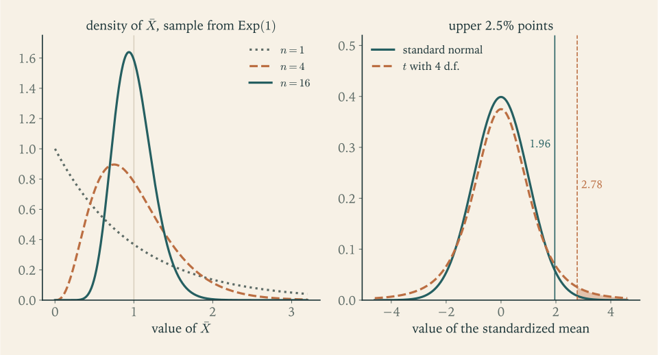
Replacing \(\sigma\) by its estimate \(S\) has a cost, and the \(t\) distribution measures it. The denominator is random, and when \(S\) happens to be small the ratio is large, so \(t_k\) has heavier tails than the standard normal. The upper \(2.5\%\) point is \(z_{0.025}=1.960\) for the normal, and it is \(2.776\) for \(t_4\) , \(2.262\) for \(t_9\) , \(2.064\) for \(t_{24}\) , and \(1.984\) for \(t_{99}\) . As the degrees of freedom grow, \(S\) becomes a precise estimate of \(\sigma\) and the \(t\) quantiles approach the normal ones.

2.3 Pivots

The variable \(\sqrt n(\bar X-\mu)/\sigma\) of Example 2.2 is not a statistic, since it involves \(\mu\) and \(\sigma\) . Its value is that its distribution is the same standard normal law for every \(\mu\) and \(\sigma\) .

A pivot packages the data and the unknown together in such a way that the uncertainty about the package is fully known. Once a pivot is in hand, any probability statement about it, such as \(P_\theta(a\le Q(X,\theta)\le b)=0.95\) , holds simultaneously for every \(\theta\) , and can be rearranged into a statement about where \(\theta\) lies relative to the data. Chapter 7 carries out that rearrangement. Here the task is to find pivots.

Theorem 2.5 and Corollary 2.6 supply three for the normal model: \(\sqrt n(\bar X-\mu)/\sigma\) , which is useful when \(\sigma\) is known; \(\sqrt n(\bar X-\mu)/S\) , which involves only \(\mu\) ; and \((n-1)S^2/\sigma^2\) , which involves only \(\sigma^2\) . That normal models yield pivots is no accident of the normal density. It comes from the location-scale structure.

The proposition says that these quantities are pivots for any \(f_0\) . It does not say their distributions are normal, chi-square, or \(t\) ; that is true only when \(f_0\) is the standard normal density. For another \(f_0\) the distribution of \(\bar Z/S_Z\) is some other fixed law, which can be tabulated by numerical integration or by simulating samples from \(f_0\) .

2.4 Order statistics and pivots that need no model

Write \(X_{(1)}\le X_{(2)}\le\dots\le X_{(n)}\) for the sample arranged in increasing order. These are the order statistics; the minimum is \(X_{(1)}\) , the maximum is \(X_{(n)}\) , and the sample median is the middle one when \(n\) is odd.

For a parametric family the proposition gives the sampling distribution of any order statistic. Its more surprising use is in models with no parametric form at all.

In the nonparametric model “random sample from a continuous \(F\) ”, the quantity \(F(X_i)\) is a pivot: it involves the unknown \(F\) , and its distribution is uniform whatever \(F\) is. So is the number of observations below any fixed quantile of \(F\) . Chapter 13 uses the same transform to check whether a forecaster’s predictive distributions are calibrated.

2.5 When the exact distribution is out of reach

For most statistics and most models no pivot with a tabulated distribution exists. The fallback is an approximation valid for large samples. The fundamental one is the Central Limit Theorem: if \(X_1,X_2,\dots\) are independent and identically distributed with mean \(\mu\) and finite positive variance \(\sigma^2\) , then \(\sqrt n(\bar X-\mu)/\sigma\) converges in distribution to the standard normal (math.probability-theory.central-limit-theorem). In the language of this chapter, \(\sqrt n(\bar X-\mu)/\sigma\) is an approximate pivot in any model with finite variance. The left panel of Figure 2.1 shows the approximation forming: the mean of exponential observations has a skewed distribution for \(n=4\) and a nearly symmetric bell shape for \(n=16\) .

The theorem is a limit statement and carries no guarantee at a given \(n\) . How large \(n\) must be depends on how far the population is from normal, chiefly on its skewness and on the weight of its tails, and the quality of the approximation is usually worst in the tails of the sampling distribution, which is where inference uses it.

Exercises

1. For the population \(\{1,2,6\}\) and samples of size two of Example 2.1, tabulate the sampling distribution of the sample maximum, compute its mean, and compare the mean with the population maximum.

   Answer

   The maximum equals \(1\) with probability \(1/9\) , equals \(2\) with probability \(3/9\) , and equals \(6\) with probability \(5/9\) . Its mean is \((1+6+30)/9=37/9\approx 4.11\) , below the population maximum \(6\) : a sample maximum can never exceed the population maximum and sometimes falls short.

2. A random sample of size \(36\) is taken from a normal population with \(\sigma=12\) . Compute the standard error of \(\bar X\) , the probability that \(\bar X\) lies within \(3\) of \(\mu\) , and the smallest sample size for which that probability is at least \(0.95\) .

   Answer

   Standard error \(12/\sqrt{36}=2\) . \(P(\lvert\bar X-\mu\rvert\le 3)=2\Phi(1.5)-1\approx 0.8664\) . The requirement \(3\sqrt n/12\ge 1.960\) gives \(n\ge 61.5\) , so \(n=62\) .

3. Let \(X_1,\dots,X_n\) be a random sample from any distribution with finite variance. Prove that \(\operatorname{Cov}(\bar X,X_i-\bar X)=0\) for each \(i\) , and explain, with reference to Example 2.1, why this does not make \(\bar X\) and \(S^2\) independent.

   Solution

   By bilinearity of covariance, \(\operatorname{Cov}(\bar X,X_i-\bar X)=\operatorname{Cov}(\bar X,X_i)-\operatorname{Var}\bar X\) . Since \(\bar X=\frac1n\sum_j X_j\) and the observations are independent, only the term \(j=i\) contributes to the first covariance: \(\operatorname{Cov}(\bar X,X_i)=\frac1n\operatorname{Var}X_i=\sigma^2/n\) . By Theorem 2.2, \(\operatorname{Var}\bar X=\sigma^2/n\) as well, so the difference is zero.

   Zero covariance says only that there is no linear association between \(\bar X\) and each residual \(X_i-\bar X\) . The sample variance is a quadratic function of the residuals, and quadratic functions of uncorrelated variables can depend strongly on one another. In Example 2.1 the event \(S^2=0\) has probability \(1/3\) and the event \(\bar X=3.5\) has probability \(2/9\) , yet they cannot occur together, so \(P(S^2=0,\ \bar X=3.5)=0\ne\tfrac13\cdot\tfrac29\) . For normal samples the vector of \(\bar X\) and the residuals is jointly normal, and for jointly normal variables zero covariance does imply independence; that is another route to the independence statement in Theorem 2.5.

4. For a random sample of size \(10\) from a normal distribution, compute \(P(S^2\le 0.5\,\sigma^2)\) and find the constant \(c\) with \(P(S^2>c\,\sigma^2)=0.05\) .

   Answer

   \(P(S^2\le 0.5\sigma^2)=P(\chi^2_9\le 4.5)\approx 0.1245\) . For the second part, \(9c=\chi^2_{9,0.05}\approx 16.919\) , so \(c\approx 1.880\) .

5. Prove that \(E\,S\le\sigma\) for every random sample from a distribution with finite variance, with strict inequality unless \(S\) is constant with probability one, and compute \(E\,S/\sigma\) exactly for a normal sample of size \(2\) .

   Solution

   For any random variable with a finite second moment, \(\operatorname{Var}(S)=E\,S^2-(E\,S)^2\ge 0\) , with equality exactly when \(S\) is constant with probability one. By Theorem 2.2, \(E\,S^2=\sigma^2\) . Hence \((E\,S)^2\le\sigma^2\) , and since \(S\ge 0\) this gives \(E\,S\le\sigma\) , with strict inequality unless \(S\) is almost surely constant. The square root is a concave function, and the result is an instance of Jensen’s inequality, stated in Section 4.5: the expectation of a concave function of a variable is at most the function of the expectation.

   For a normal sample of size \(2\) , \(S^2=(X_1-X_2)^2/2\) , so \(S=\lvert X_1-X_2\rvert/\sqrt2\) . The difference \(X_1-X_2\) is \(N(0,2\sigma^2)\) , and the mean absolute value of a \(N(0,\tau^2)\) variable is \(\tau\sqrt{2/\pi}\) . With \(\tau=\sigma\sqrt2\) ,

   \[ E\,S=\frac{\sigma\sqrt2\,\sqrt{2/\pi}}{\sqrt2}=\sigma\sqrt{\frac{2}{\pi}}\approx 0.798\,\sigma . \]

   With two observations the sample standard deviation underestimates \(\sigma\) by about \(20\%\) on average, even though \(S^2\) is exactly unbiased for \(\sigma^2\) .

6. Let \(X_1,\dots,X_m\) and \(Y_1,\dots,Y_n\) be independent random samples from \(N(\mu_1,\sigma^2)\) and \(N(\mu_2,\sigma^2)\) with a common unknown variance, and let \(S_p^2=\bigl((m-1)S_X^2+(n-1)S_Y^2\bigr)/(m+n-2)\) . Prove that \(\bigl(\bar X-\bar Y-(\mu_1-\mu_2)\bigr)/\bigl(S_p\sqrt{1/m+1/n}\bigr)\) has the \(t_{m+n-2}\) distribution.

   Solution

   Apply Theorem 2.5 to each sample. First, \(\bar X\sim N(\mu_1,\sigma^2/m)\) and \(\bar Y\sim N(\mu_2,\sigma^2/n)\) are independent, so

   \[ Z_0=\frac{\bar X-\bar Y-(\mu_1-\mu_2)}{\sigma\sqrt{1/m+1/n}}\sim N(0,1). \]

   Second, \((m-1)S_X^2/\sigma^2\sim\chi^2_{m-1}\) and \((n-1)S_Y^2/\sigma^2\sim\chi^2_{n-1}\) are independent, being functions of different samples. A sum of independent chi-square variables is chi-square with the degrees of freedom added, directly from Definition 2.3, so

   \[ V=\frac{(m+n-2)S_p^2}{\sigma^2}=\frac{(m-1)S_X^2+(n-1)S_Y^2}{\sigma^2}\sim\chi^2_{m+n-2}. \]

   Third, \(Z_0\) is independent of \(V\) : within each sample the mean is independent of the variance by Theorem 2.5, and the two samples are independent of each other, so the pair \((\bar X,\bar Y)\) is independent of the pair \((S_X^2,S_Y^2)\) . By the definition of the \(t\) distribution,

   \[ \frac{Z_0}{\sqrt{V/(m+n-2)}}=\frac{\bar X-\bar Y-(\mu_1-\mu_2)}{S_p\sqrt{1/m+1/n}}\sim t_{m+n-2}, \]

   the common \(\sigma\) having cancelled. The equal-variance assumption is what makes the cancellation possible.

7. Two independent normal samples of size \(10\) have variances \(\sigma_1^2\) and \(\sigma_2^2\) . Find a pivot involving only the ratio \(\sigma_1^2/\sigma_2^2\) , name its distribution, and compute the probability that \(S_1^2/S_2^2\) exceeds \(2.5\) when the two population variances are equal.

   Answer

   \((S_1^2/\sigma_1^2)/(S_2^2/\sigma_2^2)\sim F_{9,9}\) , a pivot involving only \(\sigma_1^2/\sigma_2^2\) . With equal variances, \(P(S_1^2/S_2^2>2.5)=P(F_{9,9}>2.5)\approx 0.0942\) .

8. In the model \(N(\mu,\sigma^2)\) with both parameters unknown, decide which of the following are pivots and justify each answer from Theorem 2.5 or Proposition 2.8: (a) \(\bar X-\mu\) ; (b) \((\bar X-\mu)/S\) ; (c) \(S^2/\sigma^2\) ; (d) \(\bar X/S\) .

   Answer

   (a) Not a pivot: its distribution \(N(0,\sigma^2/n)\) depends on \(\sigma\) . (b) A pivot: \(\sqrt n\) times it is \(t_{n-1}\) . (c) A pivot: \((n-1)\) times it is \(\chi^2_{n-1}\) . (d) Not a pivot: it is a statistic, and its distribution depends on \(\mu/\sigma\) .

9. Let \(M\) be the maximum of a random sample of size \(n\) from the uniform distribution on \((0,\theta)\) . (a) For \(n=8\) find \(a\) with \(P_\theta(a\le M/\theta\le 1)=0.95\) . (b) Show that \(n(1-M/\theta)\) converges in distribution to \(\operatorname{Exp}(1)\) as \(n\to\infty\) , and contrast the rate \(n\) with the rate \(\sqrt n\) of the Central Limit Theorem.

   Solution

   (a) As in Example 2.3, \(P_\theta(M/\theta\le u)=u^n\) for \(0\le u\le 1\) . With \(n=8\) , the requirement \(P(a\le M/\theta\le 1)=1-a^8=0.95\) gives \(a=0.05^{1/8}\approx 0.6877\) .

   (b) Fix \(t\ge 0\) . For \(n>t\) ,

   \[ P_\theta\bigl(n(1-M/\theta)>t\bigr)=P_\theta\Bigl(\frac M\theta<1-\frac tn\Bigr)=\Bigl(1-\frac tn\Bigr)^n\longrightarrow e^{-t}, \]

   which is the probability that an \(\operatorname{Exp}(1)\) variable exceeds \(t\) . Since the limit function is continuous, this is convergence in distribution.

   The scaling is by \(n\) , not \(\sqrt n\) . In the Central Limit Theorem the error \(\bar X-\mu\) is of order \(1/\sqrt n\) and its limit is normal. Here the error \(\theta-M\) is of order \(1/n\) , much smaller, and its limit is exponential, a one-sided skewed law, because the maximum can only undershoot. The uniform model has a boundary that moves with the parameter, and statistics that sit at the boundary are governed by different asymptotics from averages.

10. For a random sample of size \(n\) from \(\operatorname{Exp}(\lambda)\) , find the distribution of the minimum \(X_{(1)}\) , show that \(n\lambda X_{(1)}\) is a pivot, and explain why the pivot \(2\lambda\sum X_i\) of Example 2.4 is nevertheless preferred.

    Hint

    \(P(X_{(1)}>x)=P(\text{all } X_i>x)=e^{-n\lambda x}\) , so \(X_{(1)}\sim\operatorname{Exp}(n\lambda)\) and \(n\lambda X_{(1)}\sim\operatorname{Exp}(1)\) . Compare relative spread: the \(\operatorname{Exp}(1)\) pivot has standard deviation equal to its mean for every \(n\) , while \(\chi^2_{2n}\) has standard deviation \(2\sqrt n\) against mean \(2n\) . Which pivot pins \(\lambda\) down more tightly as \(n\) grows?

11. A report states: “Each measurement is \(N(\mu,\sigma^2)\) , so 95% of sample means of 25 measurements fall within \(\mu\pm 1.96\,\sigma\) .” Find the error, state the correct interval, and compute the actual probability that a mean of 25 falls within \(\mu\pm 1.96\,\sigma\) .

    Solution

    The error is the use of \(\sigma\) , the standard deviation of a single measurement, where the standard error of the mean is required. By Theorem 2.5 the mean of 25 measurements is \(N(\mu,\sigma^2/25)\) , with standard error \(\sigma/5\) . The interval that contains \(95\%\) of sample means is

    \[ \mu\pm 1.96\,\frac{\sigma}{5}=\mu\pm 0.392\,\sigma . \]

    The interval in the report, \(\mu\pm 1.96\,\sigma\) , is five times too wide. In units of the standard error its half-width is \(1.96\times 5=9.8\) , so the probability that a mean of 25 falls inside it is \(P(\lvert Z\rvert<9.8)\) , which differs from \(1\) by about \(10^{-22}\) . The statement in the report is therefore not false as a lower bound, but as a description of the variability of means it overstates the spread by a factor of five; the interval \(\mu\pm1.96\sigma\) describes individual measurements, not their averages.

12. A student with a normal sample of size \(5\) and unknown variance uses the cutoff \(1.96\) for \(\sqrt 5(\bar X-\mu)/S\) . Compute the actual probability that this quantity lies between \(-1.96\) and \(1.96\) , and give the cutoff that achieves probability \(0.95\) .

    Solution

    By Corollary 2.6, \(T=\sqrt5(\bar X-\mu)/S\) has the \(t_4\) distribution. The probability that \(T\) lies between \(-1.96\) and \(1.96\) is

    \[ 1-2P(t_4>1.96)\approx 0.8784 . \]

    So an interval or test built with the normal cutoff has an actual error rate of about \(12.2\%\) where \(5\%\) was intended, more than twice the nominal rate. The cutoff that gives probability \(0.95\) is the upper \(2.5\%\) point of \(t_4\) , namely \(t_{4,0.025}\approx 2.776\) . The difference between \(1.96\) and \(2.776\) is the price of estimating \(\sigma\) from five observations: the denominator \(S\) has only four degrees of freedom and is frequently much smaller than \(\sigma\) , which inflates the ratio.

13. For a random sample of size \(5\) from the uniform distribution on \((0,1)\) , find the density of the sample median, verify that it integrates to one, and compare the variance of the median with the variance of the sample mean.

    Solution

    For the uniform distribution on \((0,1)\) , \(F(x)=x\) and \(f(x)=1\) . The median of five is the third order statistic, so by Proposition 2.9 with \(n=5\) and \(k=3\) ,

    \[ f_{(3)}(x)=\frac{5!}{2!\,2!}x^2(1-x)^2=30x^2(1-x)^2,\qquad 0<x<1 . \]

    Expanding, \(30\int_0^1(x^2-2x^3+x^4)\,dx=30\bigl(\tfrac13-\tfrac12+\tfrac15\bigr)=30\cdot\tfrac1{30}=1\) . The density is symmetric about \(1/2\) , so the mean is \(1/2\) . The second moment is \(30\int_0^1(x^4-2x^5+x^6)\,dx=30\bigl(\tfrac15-\tfrac13+\tfrac17\bigr)=\tfrac{2}{7}\) , and the variance is \(\tfrac27-\tfrac14=\tfrac1{28}\approx 0.0357\) .

    The sample mean has variance \(\sigma^2/5=(1/12)/5=1/60\approx 0.0167\) . For uniform data the mean is the more precise estimator of the centre, by a factor of \(60/28\approx 2.1\) in variance. For heavy-tailed populations the comparison reverses, which is why the choice between mean and median depends on the model.

14. For a random sample of size \(10\) from a continuous distribution with median \(m\) , compute \(P(X_{(2)}<m<X_{(9)})\) and explain why the answer does not depend on the distribution.

    Answer

    The interval misses \(m\) when at most one or at least nine of the ten observations lie below \(m\) . With \(B\sim\operatorname{Binomial}(10,1/2)\) , the probability is \(1-2P(B\le 1)=1-2\cdot\tfrac{11}{1024}\approx 0.9785\) . Only the fact that each observation falls below \(m\) with probability \(1/2\) was used.

15. Show by an explicit example that Proposition 2.10 fails when \(F\) is not continuous, and identify the step of the proof that breaks.

    Hint

    Take \(X\) equal to \(0\) or \(1\) with probability \(1/2\) each. Then \(F(X)\) takes only the values \(1/2\) and \(1\) . In the proof, look at the claim \(F(x_u)=u\) for \(u=0.3\) .

16. Let \(X_1,\dots,X_{50}\) be a random sample from the Poisson distribution with mean \(2\) . Compute \(P(\bar X\ge 2.4)\) exactly, using the fact that a sum of independent Poisson variables is Poisson, and compare it with the normal approximation with and without a continuity correction.

    Answer

    \(\sum X_i\sim\operatorname{Poisson}(100)\) and \(\bar X\ge 2.4\) means \(\sum X_i\ge 120\) . Exact: \(\approx 0.0282\) . Normal without correction: \(1-\Phi(2)\approx 0.0228\) . With continuity correction: \(1-\Phi(1.95)\approx 0.0256\) . The correction removes about half the error; the rest is skewness.

17. Prove the identity \(\sum_{i=1}^n (X_i-\bar X)^2=\frac{1}{2n}\sum_{i=1}^n\sum_{j=1}^n (X_i-X_j)^2\) , and use it to give a second proof that \(E\,S^2=\sigma^2\) which never mentions \(\mu\) .

    Solution

    Write \(X_i-X_j=(X_i-\bar X)-(X_j-\bar X)\) and expand the square:

    \[ \sum_{i}\sum_{j}(X_i-X_j)^2=\sum_i\sum_j (X_i-\bar X)^2+\sum_i\sum_j (X_j-\bar X)^2-2\sum_i (X_i-\bar X)\sum_j (X_j-\bar X). \]

    Each of the first two double sums equals \(n\sum_i (X_i-\bar X)^2\) , and the last term is zero because \(\sum_i (X_i-\bar X)=0\) . Hence the double sum equals \(2n\sum_i (X_i-\bar X)^2\) , which is the identity.

    For the expectation: when \(i=j\) the term \((X_i-X_j)^2\) is zero. When \(i\ne j\) , \(X_i-X_j\) has mean zero and, by independence, variance \(2\sigma^2\) , so \(E(X_i-X_j)^2=2\sigma^2\) . There are \(n(n-1)\) ordered pairs with \(i\ne j\) . Therefore

    \[ E\sum_i (X_i-\bar X)^2=\frac{1}{2n}\cdot n(n-1)\cdot 2\sigma^2=(n-1)\sigma^2, \]

    and dividing by \(n-1\) gives \(E\,S^2=\sigma^2\) . The population mean never entered: \(S^2\) is the average over pairs of half the squared difference, and each pair on its own is an unbiased estimate of \(\sigma^2\) .

18. A sample of size \(n\) is drawn without replacement from a finite population of \(N\) values with mean \(\mu\) and variance \(\sigma^2=\frac1N\sum_k (v_k-\mu)^2\) , as in Example 1.5. Show that \(\operatorname{Cov}(X_i,X_j)=-\sigma^2/(N-1)\) for \(i\ne j\) and deduce that \(\operatorname{Var}\bar X=\frac{\sigma^2}{n}\cdot\frac{N-n}{N-1}\) .

    Hint

    Each \(X_i\) is marginally uniform on the population, so \(\operatorname{Var}X_i=\sigma^2\) . If \(n=N\) the sum \(\sum X_i\) is the population total, a constant, so its variance is zero: \(0=N\sigma^2+N(N-1)c\) where \(c\) is the common covariance. Solve for \(c\) , then expand \(\operatorname{Var}(\sum_{i\le n}X_i)=n\sigma^2+n(n-1)c\) .

19. Let \(X_i=\mu+\sigma Z_i\) where the \(Z_i\) are a random sample from the Laplace density \(\tfrac12e^{-\lvert z\rvert}\) . Explain why \(\sqrt n(\bar X-\mu)/S\) is a pivot but does not have a \(t\) distribution, and describe a procedure for obtaining its upper \(2.5\%\) point for \(n=5\) .

    Hint

    Proposition 2.8 applies with \(f_0\) the Laplace density, so the quantity is a pivot. Corollary 2.6 needs normality, which fails. Generate many samples of five from the standard Laplace density, compute \(\sqrt5\,\bar Z/S_Z\) for each, and take the empirical \(97.5\%\) point; the simulation is legitimate because the law of the pivot involves no unknowns.