Sixteen patients receive a new treatment and \(X\) of them respond. Three analysts estimate the response probability \(p\) . The first reports \(X/16\) , the observed proportion. The second reports \((X+1)/18\) , arguing that with no responders the estimate \(0\) would be absurdly confident. The third reports \((X+2)/20\) . When \(X=4\) their estimates are \(0.250\) , \(0.278\) , and \(0.300\) . Which analyst is right?
The question has no answer until “right” is given a meaning, and the natural meanings disagree. One can ask that the estimator be correct on average. One can ask that it be close to the truth, in some average sense, and then must say close under which truth, since the truth is unknown and the three estimators rank differently at different values of \(p\) . This chapter sets up the language in which such comparisons are made: bias, variance, mean squared error, and, more generally, risk. Its main conclusion is negative and important. No estimator is best for every parameter value, so every claim of optimality in statistics carries a qualification: best within a class, best in the worst case, or best on average. The chapters that follow make one of those qualifications each.
4.1 Three numbers that describe an estimator
Let \(\delta=\delta(X)\) be an estimator of a real estimand \(g(\theta)\) . Its sampling distribution, in the sense of Chapter 2, determines how it performs.
Definition 4.1 (bias, variance, mean squared error). The bias of \(\delta\) at \(\theta\) is \(b(\theta)=E_\theta\,\delta(X)-g(\theta)\) , and \(\delta\) is unbiased if \(b(\theta)=0\) for every \(\theta\in\Theta\) . The variance is \(\operatorname{Var}_\theta\,\delta(X)\) . The mean squared error is
Each is a function of \(\theta\) , not a number. Bias measures a systematic tendency to overshoot or undershoot; variance measures how much the estimator moves from sample to sample; mean squared error measures the typical squared distance from the target. They are tied together by an identity.
Theorem 4.2 (bias-variance decomposition). For any estimator \(\delta\) with finite second moment,
Proof. Write \(m=E_\theta\,\delta\) , so that \(b=m-g(\theta)\) , and split the error as \(\delta-g(\theta)=(\delta-m)+b\) . Squaring,
Take expectations. The first term gives the variance. The middle term vanishes because \(b\) is a constant and \(E_\theta(\delta-m)=0\) . The last term is the constant \(b^2\) .
The decomposition says that there are two ways to be wrong and that they add. It also shows that the two can be traded: accepting a little bias is worthwhile whenever it buys a larger reduction in variance.
Example 4.1: Three divisors for a normal variance
Let \(X_1,\dots,X_{10}\) be a random sample from \(N(\mu,\sigma^2)\) and write \(W=\sum(X_i-\bar X)^2\) . Consider estimators of \(\sigma^2\) of the form \(cW\) . By Theorem 2.5, \(W/\sigma^2\sim\chi^2_9\) , with mean \(9\) and variance \(18\) . Hence
Three choices of \(c\) are in common use.
| Divisor | Bias | Variance | Mean squared error |
|---|---|---|---|
| \(9\) , the sample variance \(S^2\) | \(0\) | \(\tfrac{2}{9}\sigma^4\approx 0.2222\,\sigma^4\) | \(0.2222\,\sigma^4\) |
| \(10\) | \(-\tfrac{1}{10}\sigma^2\) | \(0.18\,\sigma^4\) | \(0.19\,\sigma^4\) |
| \(11\) | \(-\tfrac{2}{11}\sigma^2\) | \(\tfrac{18}{121}\sigma^4\approx 0.1488\,\sigma^4\) | \(\tfrac{2}{11}\sigma^4\approx 0.1818\,\sigma^4\) |
The unbiased estimator has the largest mean squared error of the three, for every value of \(\mu\) and \(\sigma^2\) . Minimising \(18c^2+(9c-1)^2\) over \(c\) gives \(c=1/11\) : dividing by \(n+1\) is the best choice of this form, and its mean squared error is about \(18\%\) smaller than that of \(S^2\) . Shrinking the estimate toward zero reduces variance by more than the squared bias it introduces. Whether that settles the matter depends on whether mean squared error is the right criterion; someone who will average many such estimates across studies has a reason to prefer the unbiased one, because biases accumulate under averaging and variances do not.
4.2 Where estimators come from
Before comparing estimators one needs some to compare. Two general recipes produce most of them. Maximum likelihood is the subject of Chapter 5. The older and simpler one matches moments.
Definition 4.3 (method of moments). Let \(X_1,\dots,X_n\) be a random sample from a model with \(k\) -dimensional parameter \(\theta\) , and suppose the first \(k\) population moments \(m_j(\theta)=E_\theta X^j\) exist. The method-of-moments estimator \(\tilde\theta\) is a solution of the \(k\) equations
The idea is the plug-in principle: sample moments estimate population moments, so solve for the parameter values that make the two agree. The method needs no density, only formulas for moments, and it almost always yields an explicit answer. Its estimators are not generally functions of a minimal sufficient statistic, and that is a warning that information may be wasted.
Example 4.2: Fitting a gamma distribution by moments
Eight failure times, in thousands of hours, are \(1.2\) , \(0.8\) , \(2.6\) , \(1.9\) , \(0.5\) , \(3.1\) , \(1.4\) , \(2.5\) , modelled as a random sample from \(\operatorname{Gamma}(a,b)\) . The mean of the gamma distribution is \(a/b\) and its variance is \(a/b^2\) . Matching the first two moments is the same as matching the mean and the variance with divisor \(n\) :
Dividing the first equation by the second gives \(\tilde b=1.75/0.7525\approx 2.326\) , and then \(\tilde a=\bar x\,\tilde b=1.75^2/0.7525\approx 4.070\) . The fitted distribution has shape about \(4.07\) and rate about \(2.33\) per thousand hours. The maximum likelihood estimator for the same model has no closed form and must be computed numerically, which is the typical trade: moments are easy, likelihood is efficient.
Example 4.3: Two estimators of a uniform endpoint
Let \(X_1,\dots,X_n\) be a random sample from the uniform distribution on \((0,\theta)\) . Since \(E_\theta X=\theta/2\) , the method-of-moments estimator is \(\tilde\theta=2\bar X\) . It is unbiased, with variance \(4\cdot\frac{\theta^2}{12n}=\theta^2/(3n)\) .
The sufficient statistic is the maximum \(M\) , whose density is \(nm^{n-1}/\theta^n\) on \((0,\theta)\) . Direct integration gives \(E_\theta M=\frac{n}{n+1}\theta\) and \(E_\theta M^2=\frac{n}{n+2}\theta^2\) . So \(M\) is biased downward, and
Correcting the bias gives \(\hat\theta=\frac{n+1}{n}M\) , which is unbiased with variance \(\theta^2/(n(n+2))\) . For \(n=10\) :
The estimator built on the sufficient statistic has one quarter of the mean squared error of the moment estimator, and the gap widens with \(n\) , because its variance falls like \(1/n^2\) and the other’s like \(1/n\) . Even the biased raw maximum beats the unbiased \(2\bar X\) .
The moment estimator has a second defect. For the data \(0.3\) , \(0.5\) , \(0.4\) , \(3.0\) , \(0.8\) it gives \(2\bar x=2.0\) , although an observation of \(3.0\) proves that \(\theta\) is at least \(3\) . An estimate that the data themselves contradict is a sign that the method has ignored part of the model.
4.3 Loss, risk, and why no estimator is best everywhere
Squared error is one way to score a mistake. The general framework replaces it by an arbitrary penalty.
Definition 4.4 (loss and risk). A loss function \(L(\theta,d)\ge 0\) gives the penalty for estimating \(g(\theta)\) by the value \(d\) . The risk function of an estimator \(\delta\) is its expected loss,
Under squared error loss \(L(\theta,d)=(d-g(\theta))^2\) the risk is the mean squared error. Under absolute error loss \(L(\theta,d)=\lvert d-g(\theta)\rvert\) it is the mean absolute error. An asymmetric loss is appropriate when overestimating and underestimating have different consequences, as when the estimate sets the size of an order or the dose of a drug. The risk is a function of \(\theta\) , and comparing two estimators means comparing two functions.
Definition 4.5 (domination and admissibility). An estimator \(\delta_1\) dominates \(\delta_2\) if \(R(\theta,\delta_1)\le R(\theta,\delta_2)\) for every \(\theta\in\Theta\) , with strict inequality for at least one \(\theta\) . An estimator is inadmissible if some estimator dominates it, and admissible otherwise.
In Example 4.1 the estimator with divisor \(11\) dominates \(S^2\) under squared error loss, so \(S^2\) is inadmissible for that loss. In Example 4.3 the estimator \(\frac{n+1}{n}M\) dominates \(2\bar X\) whenever \(n\ge2\) . Domination is the one unambiguous comparison: a dominated estimator should not be used for the loss in question. Usually, though, neither of two estimators dominates the other, and there is a structural reason.
Proposition 4.6 (no uniformly best estimator). Suppose there are \(\theta_1,\theta_2\in\Theta\) with \(g(\theta_1)\ne g(\theta_2)\) such that \(P_{\theta_1}\) and \(P_{\theta_2}\) assign probability zero to the same events. Then no estimator \(\delta^\ast\) satisfies \(\operatorname{MSE}_\theta(\delta^\ast)\le\operatorname{MSE}_\theta(\delta)\) for all \(\theta\) and all estimators \(\delta\) .
Proof. Suppose such a \(\delta^\ast\) existed. The constant estimator \(\delta_1\equiv g(\theta_1)\) has mean squared error zero at \(\theta_1\) , so \(\operatorname{MSE}_{\theta_1}(\delta^\ast)=0\) , which forces \(\delta^\ast(X)=g(\theta_1)\) with \(P_{\theta_1}\) -probability one. By the same argument with the constant \(g(\theta_2)\) , \(\delta^\ast(X)=g(\theta_2)\) with \(P_{\theta_2}\) -probability one. The event \(\{\delta^\ast(X)\ne g(\theta_1)\}\) has \(P_{\theta_1}\) -probability zero, hence \(P_{\theta_2}\) -probability zero by hypothesis. Then under \(P_{\theta_2}\) the estimator equals both \(g(\theta_1)\) and \(g(\theta_2)\) with probability one, contradicting \(g(\theta_1)\ne g(\theta_2)\) .
The constant estimator used in the proof is a foolish one: it ignores the data and is excellent only if the guess happens to be right. Yet it cannot be beaten at its favoured parameter value, and it is admissible (Exercise 7). The proposition shows that asking for the smallest risk everywhere is asking for too much, and admissibility alone is asking for too little.
Example 4.4: Three analysts, three risk curves
Return to the opening, with \(X\sim\operatorname{Binomial}(16,p)\) . For an estimator of the form \((X+a)/(16+2a)\) the mean is \((16p+a)/(16+2a)\) , so the bias is \(a(1-2p)/(16+2a)\) and the variance is \(16p(1-p)/(16+2a)^2\) . By Theorem 4.2,
The three analysts use \(a=0\) , \(a=1\) , and \(a=2\) :
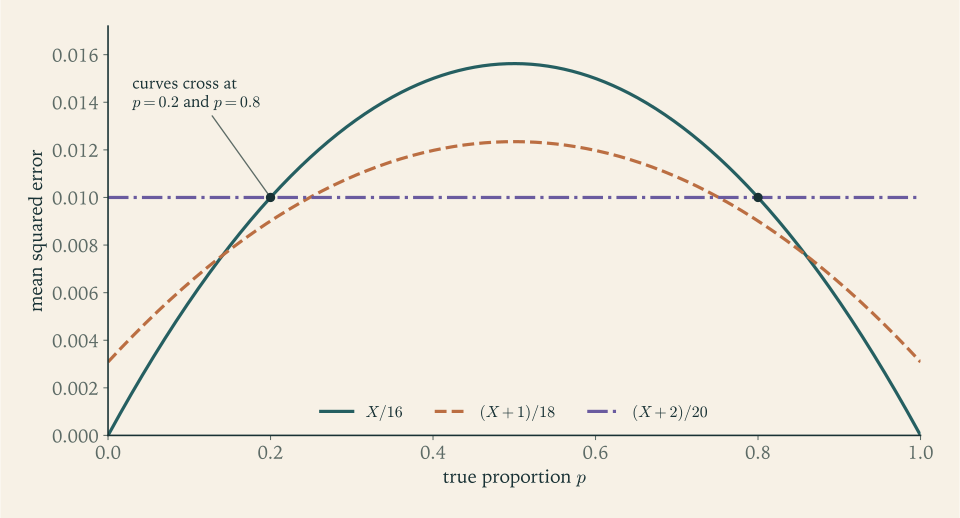
The last simplification holds because \(16p(1-p)+4(1-4p+4p^2)=4\) for every \(p\) : the third analyst’s estimator has constant risk \(0.01\) . The first has risk zero at \(p=0\) and \(p=1\) and maximum risk \(1/64\approx 0.0156\) at \(p=1/2\) . The second has maximum risk \(1/81\approx 0.0123\) at \(p=1/2\) and risk \(1/324\approx 0.0031\) at the endpoints.
Solving \(R_0(p)=R_2(p)\) gives \(p(1-p)=0.16\) , that is, \(p=0.2\) or \(p=0.8\) . So the observed proportion is better than the constant-risk estimator when \(p\) is below \(0.2\) or above \(0.8\) , and worse in between. The curves \(R_0\) and \(R_1\) cross at \(p\approx 0.141\) and \(p\approx 0.859\) , and \(R_1\) and \(R_2\) cross at \(p\approx 0.248\) and \(p\approx 0.752\) . Each estimator is the best of the three on some range of \(p\) , and none dominates another.
4.4 Turning a risk function into a number
Since risk functions cross, a choice among estimators requires an additional principle. Two principles reduce each risk function to a single number so that numbers can be compared.
Definition 4.7 (minimax and average risk). The maximum risk of \(\delta\) is \(\sup_{\theta\in\Theta}R(\theta,\delta)\) , and an estimator is minimax if it minimises the maximum risk among all estimators. Given a nonnegative weight function \(w\) on \(\Theta\) with \(\int_\Theta w(\theta)\,d\theta=1\) , the average risk of \(\delta\) with respect to \(w\) is \(\int_\Theta R(\theta,\delta)\,w(\theta)\,d\theta\) .
The minimax principle protects against the worst case. It is cautious, sometimes excessively so, since it lets the least favourable parameter value dictate the choice even if that value is implausible. The average-risk principle expresses a judgment about which parameter values matter more. When the weight \(w\) is interpreted as a probability distribution for \(\theta\) , average risk is called Bayes risk, and Chapter 11 shows how to find the estimator that minimises it.
For the three estimators of Example 4.4 the two principles give different verdicts. The maximum risks are \(1/64\approx 0.0156\) , \(1/81\approx 0.0123\) , and \(1/100\) , so by the worst-case criterion the constant-risk estimator \((X+2)/20\) is the best of the three. With the uniform weight \(w(p)=1\) on \((0,1)\) , and using \(\int_0^1p(1-p)\,dp=1/6\) and \(\int_0^1(1-2p)^2\,dp=1/3\) , the average risks are
so by the uniform-average criterion \((X+1)/18\) is the best of the three. Neither verdict is an accident. Chapter 11 proves that \((X+1)/18\) minimises the uniform-average risk among all estimators, and that \((X+2)/20\) is minimax among all estimators, the latter because its risk is constant and it is an average-risk minimiser for a suitable weight. In general the estimator \((X+\sqrt n/2)/(n+\sqrt n)\) has constant risk \(n/\bigl(4(n+\sqrt n)^2\bigr)\) , and \(\sqrt{16}/2=2\) explains the third analyst’s choice.
The observed proportion is neither minimax nor optimal for the uniform average, and yet it is what most people would report. Its justification is of a third kind, taken up next.
4.5 Unbiasedness as a restriction, and its limits
A third way to escape Proposition 4.6 is to restrict the class of estimators so that the foolish constant estimators are excluded, and then look for the best member of the restricted class. The classical restriction is unbiasedness. Among unbiased estimators the mean squared error equals the variance, and there is often one with the smallest variance at every \(\theta\) simultaneously; Chapter 6 shows how to find it. In the binomial model \(X/n\) is that estimator.
Unbiasedness is attractive, since it says the estimator has no systematic tendency, but it should not be mistaken for a requirement of good estimation. It has four limitations.
It can cost accuracy. Example 4.1 exhibited a biased estimator with smaller mean squared error than the unbiased one at every parameter value.
It is not preserved by transformations. If \(\delta\) is unbiased for \(\theta\) and has positive variance, then \(E\,\delta^2=\theta^2+\operatorname{Var}\delta>\theta^2\) , so \(\delta^2\) overestimates \(\theta^2\) . Likewise \(S\) underestimates \(\sigma\) although \(S^2\) is unbiased for \(\sigma^2\) : for a normal sample \(E\,S=c_n\sigma\) with \(c_5\approx 0.940\) and \(c_{10}\approx 0.973\) . Both are instances of Jensen’s inequality from Probability Theory: if \(g\) is convex on an interval containing the values of a random variable \(Y\) with finite mean, then \(E\,g(Y)\ge g(E\,Y)\) , with strict inequality when \(g\) is strictly convex and \(Y\) is not constant; for concave \(g\) the inequality is reversed. Unbiasedness is a property of an estimator together with a particular scale for the estimand.
An unbiased estimator may not exist. In the binomial model, an estimator \(\delta(X)\) has expectation \(\sum_{x=0}^n\delta(x)\binom nx p^x(1-p)^{n-x}\) , a polynomial in \(p\) of degree at most \(n\) . Only such polynomials can be estimated without bias. The function \(1/p\) is unbounded as \(p\to 0\) and so is not a polynomial on \((0,1)\) ; no unbiased estimator of \(1/p\) exists. The same holds for the odds \(p/(1-p)\) and for \(\sqrt p\) .
The only unbiased estimator may be absurd. That is the point of the last example.
Example 4.5: An unbiased estimator nobody would use
Let \(X\) be a single Poisson observation with mean \(\lambda\) , and suppose the estimand is \(e^{-2\lambda}\) , the probability that two further independent counts would both be zero. An estimator \(\delta(X)\) is unbiased when
Two power series that agree on an interval have the same coefficients, so \(\delta(x)=(-1)^x\) is the only unbiased estimator. It estimates a probability, a number between \(0\) and \(1\) , by \(+1\) when the count is even and by \(-1\) when the count is odd. Its mean squared error is \(E\,\delta^2-(e^{-2\lambda})^2=1-e^{-4\lambda}\) , which at \(\lambda=1\) is about \(0.982\) .
The biased estimator \(e^{-2X}\) , obtained by substituting \(X\) for \(\lambda\) , always lies in \((0,1]\) . Using \(E\,e^{tX}=\exp(\lambda(e^{t}-1))\) , its mean at \(\lambda=1\) is \(\exp(e^{-2}-1)\approx 0.421\) against a target of \(e^{-2}\approx 0.135\) , so its bias is substantial, and its mean squared error is
That is poor, since one observation says little about \(e^{-2\lambda}\) , but it is less than a third of the mean squared error of the unbiased estimator. Insisting on unbiasedness here leaves a single candidate, and it is a bad one.
Common mistake. Treating “unbiased” as a synonym for “accurate”. Bias describes the centre of the sampling distribution and nothing else. An unbiased estimator with a large variance is usually far from the target, and a slightly biased estimator with a small variance is usually close.
The practical upshot of the chapter is a discipline for reporting. An estimate should come with an estimate of its standard error, and with its bias if that is not negligible. For the observed proportion the standard error is \(\sqrt{p(1-p)/n}\) , estimated by substituting \(\hat p\) for \(p\) ; Exercise 16 examines that substitution. A comparison between estimators should say which loss, and which summary of the risk function, it rests on.
Two questions remain. Where does a good estimator come from in a model more complicated than these, and in what precise sense can an unbiased estimator be best? The next two chapters answer them in turn.
Exercises
-
Let \(X\sim\operatorname{Binomial}(n,p)\) . Derive the bias, variance, and mean squared error of \(X/n\) and of \((X+1)/(n+2)\) as functions of \(p\) , and evaluate both mean squared errors at \(n=4\) , \(p=0.5\) .
Answer
\(X/n\) : bias \(0\) , variance and mean squared error \(p(1-p)/n\) . \((X+1)/(n+2)\) : bias \((1-2p)/(n+2)\) , variance \(np(1-p)/(n+2)^2\) , mean squared error \(\bigl(np(1-p)+(1-2p)^2\bigr)/(n+2)^2\) . At \(n=4\) , \(p=0.5\) : \(0.0625\) and \(1/36\approx 0.0278\) .
-
Let \(\delta_1\) and \(\delta_2\) be independent unbiased estimators of \(\theta\) with variances \(v_1\) and \(v_2\) . Show that \(a\delta_1+(1-a)\delta_2\) is unbiased for every \(a\) , find the \(a\) that minimises its variance, and show that the minimal variance is \(v_1v_2/(v_1+v_2)\) .
Solution
Unbiasedness: \(E[a\delta_1+(1-a)\delta_2]=a\theta+(1-a)\theta=\theta\) for every real \(a\) , by linearity.
Variance: by independence,
\[ V(a)=\operatorname{Var}\bigl(a\delta_1+(1-a)\delta_2\bigr)=a^2v_1+(1-a)^2v_2 . \]This is a convex quadratic in \(a\) . Setting \(V'(a)=2av_1-2(1-a)v_2=0\) gives
\[ a^\ast=\frac{v_2}{v_1+v_2},\qquad 1-a^\ast=\frac{v_1}{v_1+v_2}. \]Each estimator is weighted by the other’s variance, or equivalently in proportion to its own precision \(1/v_i\) . Substituting,
\[ V(a^\ast)=\frac{v_2^2v_1+v_1^2v_2}{(v_1+v_2)^2}=\frac{v_1v_2(v_1+v_2)}{(v_1+v_2)^2}=\frac{v_1v_2}{v_1+v_2}. \]Since \(\frac{v_1v_2}{v_1+v_2}<\min(v_1,v_2)\) , the combination is strictly better than either estimator alone, however poor the worse one is. In terms of precisions the result reads \(1/V(a^\ast)=1/v_1+1/v_2\) : precisions of independent unbiased estimators add under optimal weighting. The same weighting reappears in the posterior mean of Chapter 11.
-
For a random sample of size \(n\) from the uniform distribution on \((0,\theta)\) with maximum \(M\) , find the constant \(c\) that minimises the mean squared error of \(cM\) , give the minimal value, and compare it for \(n=10\) with the three values in Example 4.3.
Solution
From Example 4.3, \(E_\theta M=\frac{n}{n+1}\theta\) and \(E_\theta M^2=\frac{n}{n+2}\theta^2\) . Hence
\[ \operatorname{MSE}_\theta(cM)=c^2E_\theta M^2-2c\,\theta E_\theta M+\theta^2=\theta^2\Bigl[\frac{n}{n+2}c^2-\frac{2n}{n+1}c+1\Bigr]. \]The bracket is a convex quadratic in \(c\) , minimised where \(\frac{2n}{n+2}c=\frac{2n}{n+1}\) , that is, at
\[ c^\ast=\frac{n+2}{n+1}. \]The minimal value is
\[ \theta^2\Bigl[1-\frac{n}{n+1}\cdot\frac{n+2}{n+1}\Bigr]=\theta^2\,\frac{(n+1)^2-n(n+2)}{(n+1)^2}=\frac{\theta^2}{(n+1)^2}. \]For \(n=10\) this is \(\theta^2/121\approx 0.00826\,\theta^2\) , slightly below the value \(0.00833\,\theta^2\) of the unbiased estimator \(\frac{11}{10}M\) , and far below \(0.0152\,\theta^2\) for \(M\) and \(0.0333\,\theta^2\) for \(2\bar X\) . The best multiple, \(\frac{12}{11}M\) , is biased: it is a little smaller than the unbiased multiple, trading a small bias for a small variance reduction. The gain is under one percent, which is a reminder that an unbiased estimator can be inadmissible and still be nearly optimal.
-
Find the method-of-moments estimators of \(a\) and \(b\) for a random sample from the uniform distribution on \((a,b)\) , expressing them through \(\bar x\) and the variance with divisor \(n\) .
Answer
The mean is \((a+b)/2\) and the variance is \((b-a)^2/12\) . With \(v=\frac1n\sum(x_i-\bar x)^2\) : \(\tilde a=\bar x-\sqrt{3v}\) and \(\tilde b=\bar x+\sqrt{3v}\) .
-
For a random sample from the Poisson distribution, both \(\bar X\) and \(S^2\) are unbiased estimators of \(\lambda\) . Explain, using sufficiency, which you expect to be more precise, and confirm it by comparing \(\operatorname{Var}\bar X\) with the large-sample approximation \(\operatorname{Var}S^2\approx(\lambda+2\lambda^2)/n\) .
Hint
The sufficient statistic is \(\sum X_i\) , and \(\bar X\) is a function of it while \(S^2\) is not. Compare \(\lambda/n\) with \((\lambda+2\lambda^2)/n\) : the ratio is \(1+2\lambda\) , so \(S^2\) is always worse and much worse for large \(\lambda\) .
-
For a random sample of size \(n\) from \(N(\mu,\sigma^2)\) and \(W=\sum(X_i-\bar X)^2\) , derive the mean squared error of \(cW\) as an estimator of \(\sigma^2\) for general \(n\) and \(c\) , and prove that it is minimised at \(c=1/(n+1)\) .
Solution
By Theorem 2.5, \(W/\sigma^2\sim\chi^2_{n-1}\) , which has mean \(n-1\) and variance \(2(n-1)\) . Therefore \(E(cW)=c(n-1)\sigma^2\) , the bias is \((c(n-1)-1)\sigma^2\) , and \(\operatorname{Var}(cW)=2c^2(n-1)\sigma^4\) . By Theorem 4.2,
\[ \operatorname{MSE}(cW)=\sigma^4\,q(c),\qquad q(c)=2(n-1)c^2+\bigl((n-1)c-1\bigr)^2 . \]Expanding, \(q(c)=(n-1)(n+1)c^2-2(n-1)c+1\) , a convex quadratic. Its derivative \(2(n-1)(n+1)c-2(n-1)\) vanishes at
\[ c^\ast=\frac{1}{n+1}, \]and since the leading coefficient is positive this is the global minimum. The minimal value is \(q(c^\ast)=\frac{n-1}{n+1}-\frac{2(n-1)}{n+1}+1=\frac{2}{n+1}\) , so the best estimator of this form has mean squared error \(2\sigma^4/(n+1)\) , compared with \(q\bigl(\frac1{n-1}\bigr)\sigma^4=2\sigma^4/(n-1)\) for \(S^2\) . The factor \(\sigma^4\) is common to all \(c\) , so the ordering holds for every parameter value: \(W/(n+1)\) dominates \(S^2\) under squared error loss, and \(S^2\) is inadmissible for that loss.
-
Let \(X\sim\operatorname{Binomial}(n,p)\) with \(p\in(0,1)\) and fix \(p_0\in(0,1)\) . Prove that the constant estimator \(\delta\equiv p_0\) is admissible under squared error loss, and comment on what this says about admissibility as a criterion.
Solution
Suppose an estimator \(\delta'\) satisfied \(\operatorname{MSE}_p(\delta')\le\operatorname{MSE}_p(\delta)=(p_0-p)^2\) for all \(p\in(0,1)\) . At \(p=p_0\) the right side is zero, so
\[ E_{p_0}\bigl(\delta'(X)-p_0\bigr)^2=\sum_{x=0}^n\bigl(\delta'(x)-p_0\bigr)^2\binom nx p_0^x(1-p_0)^{n-x}=0 . \]Every term is nonnegative, and since \(0<p_0<1\) every binomial probability is strictly positive. Hence \(\delta'(x)=p_0\) for each \(x=0,1,\dots,n\) : the competitor is the same estimator as \(\delta\) . Then its risk equals that of \(\delta\) everywhere and the strict inequality required for domination never occurs. So nothing dominates \(\delta\) , and \(\delta\) is admissible.
This shows how weak admissibility is. An estimator that ignores the data entirely is admissible, because it is unbeatable at the one parameter value it happens to guess. Admissibility rules out estimators that are needlessly bad; it does not certify that an estimator is good. The argument is the same one used in the proof of Proposition 4.6.
-
A report asserts: “Since \(\bar X\) is unbiased for \(\mu\) , the statistic \(\bar X^2\) is unbiased for \(\mu^2\) .” Compute the bias of \(\bar X^2\) for a random sample with variance \(\sigma^2\) , and construct an unbiased estimator of \(\mu^2\) from \(\bar X\) and \(S^2\) .
Solution
By Theorem 2.2, \(E\,\bar X=\mu\) and \(\operatorname{Var}\bar X=\sigma^2/n\) . For any variable, \(E\,Y^2=\operatorname{Var}Y+(E\,Y)^2\) , so
\[ E\,\bar X^2=\mu^2+\frac{\sigma^2}{n}. \]The bias of \(\bar X^2\) as an estimator of \(\mu^2\) is \(\sigma^2/n\) , which is strictly positive whenever \(\sigma^2>0\) . The report’s claim is false: squaring is not linear, and unbiasedness passes only through linear maps.
To remove the bias, subtract an unbiased estimator of it. Since \(E\,S^2=\sigma^2\) ,
\[ E\Bigl[\bar X^2-\frac{S^2}{n}\Bigr]=\mu^2+\frac{\sigma^2}{n}-\frac{\sigma^2}{n}=\mu^2 , \]so \(\bar X^2-S^2/n\) is unbiased for \(\mu^2\) , for any population with finite variance. It has a defect of its own: it is negative whenever \(\bar X^2<S^2/n\) , and a negative estimate of the nonnegative quantity \(\mu^2\) is not credible. Truncating it at zero would repair the range and reintroduce bias.
-
In the setting of Example 4.5, verify by direct summation that \(E_\lambda(-1)^X=e^{-2\lambda}\) , derive the mean squared errors of \((-1)^X\) and of \(e^{-2X}\) as functions of \(\lambda\) , and evaluate both at \(\lambda=1\) .
Solution
Direct summation:
\[ E_\lambda(-1)^X=\sum_{x=0}^\infty(-1)^x\frac{e^{-\lambda}\lambda^x}{x!}=e^{-\lambda}\sum_{x=0}^\infty\frac{(-\lambda)^x}{x!}=e^{-\lambda}e^{-\lambda}=e^{-2\lambda}. \]Since \(\bigl((-1)^X\bigr)^2=1\) , the variance, which equals the mean squared error for an unbiased estimator, is \(1-e^{-4\lambda}\) . At \(\lambda=1\) it is \(1-e^{-4}\approx 0.982\) .
For \(e^{-2X}\) use the Poisson generating function \(E\,e^{tX}=\exp(\lambda(e^t-1))\) with \(t=-2\) and \(t=-4\) :
\[ E\,e^{-2X}=\exp\bigl(\lambda(e^{-2}-1)\bigr),\qquad E\,e^{-4X}=\exp\bigl(\lambda(e^{-4}-1)\bigr). \]Expanding the square,
\[ \operatorname{MSE}_\lambda(e^{-2X})=\exp\bigl(\lambda(e^{-4}-1)\bigr)-2e^{-2\lambda}\exp\bigl(\lambda(e^{-2}-1)\bigr)+e^{-4\lambda}. \]At \(\lambda=1\) : \(0.3747-2(0.1353)(0.4212)+0.0183\approx 0.279\) . The plug-in estimator has a bias of about \(0.4212-0.1353=0.286\) , and nevertheless its mean squared error is well under a third of that of the unbiased estimator, whose values \(\pm1\) are never within \(0.86\) of the target.
-
Let \(X\sim\operatorname{Binomial}(n,p)\) with \(n\ge 2\) . Show that \(X(n-X)/(n(n-1))\) is an unbiased estimator of \(p(1-p)\) , and show that no unbiased estimator of the odds \(p/(1-p)\) exists.
Hint
Compute \(E\,X(n-X)=nE\,X-E\,X^2\) using \(E\,X^2=np(1-p)+n^2p^2\) . For the odds, the expectation of any estimator is a polynomial in \(p\) and is therefore bounded on \((0,1)\) ; the odds are not.
-
For a random sample of size \(n\) from \(N(\mu,1)\) , compute the risk function of \(\bar X\) under absolute error loss, and evaluate it for \(n=25\) .
Answer
\(\bar X-\mu\sim N(0,1/n)\) , and the mean absolute value of \(N(0,\tau^2)\) is \(\tau\sqrt{2/\pi}\) , so the risk is \(\sqrt{2/(\pi n)}\) for every \(\mu\) . For \(n=25\) it is about \(0.160\) .
-
For a single Bernoulli observation \(X\) with success probability \(p\) , an estimator is a pair \((\delta(0),\delta(1))=(a,b)\) . Show that the choice \((1/4,3/4)\) has constant mean squared error and find the constant; compare with the maximum risk of the choice \((0,1)\) .
Answer
\((1-p)(\tfrac14-p)^2+p(\tfrac34-p)^2=\tfrac1{16}\) for every \(p\) . The choice \((0,1)\) has risk \(p(1-p)\) with maximum \(\tfrac14\) , four times as large.
-
For \(X\sim\operatorname{Binomial}(4,p)\) , compute the maximum risk and the uniform-average risk under squared error for \(X/4\) and for \((X+1)/6\) , and say which estimator each criterion prefers.
Answer
\(X/4\) : risk \(p(1-p)/4\) , maximum \(1/16=0.0625\) , uniform average \(1/24\approx 0.0417\) . \((X+1)/6\) : risk \(\bigl(4p(1-p)+(1-2p)^2\bigr)/36=1/36\approx 0.0278\) , constant, so its maximum and average are both \(1/36\) . Both criteria prefer \((X+1)/6\) ; it still does not dominate \(X/4\) , whose risk is smaller when \(p(1-p)<1/9\) .
-
Using the crossing points computed in Example 4.4, state for each of the three estimators the set of values of \(p\) on which it has the smallest mean squared error of the three.
Answer
\(X/16\) is best for \(p<0.141\) and \(p>0.859\) . \((X+1)/18\) is best for \(0.141<p<0.248\) and \(0.752<p<0.859\) . \((X+2)/20\) is best for \(0.248<p<0.752\) .
-
In the finite-lot model of Example 1.5, with a lot of \(N\) items of which \(D\) are defective and a sample of \(n\) drawn without replacement, show that \(NX/n\) is an unbiased estimator of \(D\) , find its variance, and evaluate its standard error for \(N=50\) , \(n=10\) , \(D=10\) .
Answer
\(E\,X=nD/N\) , so \(E[NX/n]=D\) . \(\operatorname{Var}(NX/n)=\frac{N^2}{n}\cdot\frac DN\bigl(1-\frac DN\bigr)\cdot\frac{N-n}{N-1}\) . For \(N=50\) , \(n=10\) , \(D=10\) the variance is about \(32.65\) and the standard error about \(5.71\) items.
-
Let \(\hat p=X/n\) with \(X\sim\operatorname{Binomial}(n,p)\) . Compute \(E\,\hat p(1-\hat p)\) , show that \(\hat p(1-\hat p)/n\) underestimates the variance of \(\hat p\) on average, and give the unbiased estimator of that variance.
Solution
Write \(\hat p(1-\hat p)=\hat p-\hat p^2\) . Since \(E\,\hat p=p\) and \(E\,\hat p^2=\operatorname{Var}\hat p+p^2=p(1-p)/n+p^2\) ,
\[ E\,\hat p(1-\hat p)=p-p^2-\frac{p(1-p)}{n}=p(1-p)\Bigl(1-\frac1n\Bigr)=\frac{n-1}{n}\,p(1-p). \]The variance of \(\hat p\) is \(p(1-p)/n\) . The plug-in estimate \(\hat p(1-\hat p)/n\) has expectation \(\frac{n-1}{n}\cdot\frac{p(1-p)}{n}\) , which is smaller than the true variance by the factor \((n-1)/n\) . So the usual estimated standard error is, on average, slightly too small, and the shortfall is the same \(n-1\) versus \(n\) phenomenon as for the sample variance: \(\hat p(1-\hat p)\) is the variance with divisor \(n\) of the \(n\) zero-one observations.
Multiplying by \(n/(n-1)\) removes the bias: \(\hat p(1-\hat p)/(n-1)\) is an unbiased estimator of \(\operatorname{Var}\hat p\) . For \(n=16\) the correction is about \(6.7\%\) in variance; for \(n=1000\) it is negligible.
-
Let \(\delta\) be an unbiased estimator of \(\theta>0\) that is positive with probability one and has positive variance. Prove that \(1/\delta\) overestimates \(1/\theta\) on average and that \(\log\delta\) underestimates \(\log\theta\) on average.
Hint
The function \(x\mapsto 1/x\) is strictly convex on \((0,\infty)\) and \(x\mapsto\log x\) is strictly concave. Apply Jensen’s inequality as stated in Section 4.5, and note that positive variance means \(\delta\) is not constant, which makes the inequality strict.
-
(a) For the binomial model with both the number of trials \(k\) and the success probability \(p\) unknown, derive the method-of-moments estimators from a random sample of counts. (b) Apply them to the counts \(0\) , \(5\) , \(1\) , \(6\) , \(2\) and explain what the result reveals about the method.
Solution
(a) A binomial count with \(k\) trials has mean \(kp\) and variance \(kp(1-p)\) . Matching the first two moments is equivalent to matching the mean \(\bar x\) and the variance \(v=\frac1n\sum(x_i-\bar x)^2\) :
\[ kp=\bar x,\qquad kp(1-p)=v . \]Dividing, \(1-p=v/\bar x\) , so
\[ \tilde p=1-\frac{v}{\bar x},\qquad \tilde k=\frac{\bar x}{\tilde p}=\frac{\bar x^2}{\bar x-v}. \](b) For the counts \(0,5,1,6,2\) : \(\bar x=14/5=2.8\) and \(v=\tfrac15(7.84+4.84+3.24+10.24+0.64)=5.36\) . Then
\[ \tilde p=1-\frac{5.36}{2.8}\approx -0.914,\qquad \tilde k=\frac{2.8^2}{2.8-5.36}\approx -3.06 . \]A negative probability and a negative number of trials are not estimates of anything. The equations have a solution, but it lies outside the parameter space. This happens whenever the sample variance exceeds the sample mean, which a binomial distribution never allows in the population, since \(kp(1-p)<kp\) . The method of moments solves equations without regard to the constraints of the model. The data here are more dispersed than any binomial distribution, and the honest conclusions are that the binomial model fits poorly or that five counts are too few to estimate \(k\) ; the moment equations report neither.
-
Let \(\bar X\sim N(\mu,1)\) and consider the shrinkage estimators \(c\bar X\) of \(\mu\) for \(0\le c\le 1\) . Find the mean squared error as a function of \(c\) and \(\mu\) , the value of \(c\) that minimises it for a given \(\mu\) , and the set of \(\mu\) for which \(c=0.8\) beats \(c=1\) . Explain why the minimising \(c\) is not an estimator.
Solution
\(c\bar X\) has mean \(c\mu\) , bias \((c-1)\mu\) , and variance \(c^2\) . By Theorem 4.2,
\[ \operatorname{MSE}_\mu(c\bar X)=c^2+(1-c)^2\mu^2 . \]For fixed \(\mu\) this is a convex quadratic in \(c\) with derivative \(2c-2(1-c)\mu^2\) , which vanishes at
\[ c^\ast(\mu)=\frac{\mu^2}{1+\mu^2}. \]For \(c=0.8\) the mean squared error is \(0.64+0.04\mu^2\) , and for \(c=1\) it is \(1\) . So \(c=0.8\) is better exactly when \(0.04\mu^2<0.36\) , that is, when \(\lvert\mu\rvert<3\) . Outside that range the bias of the shrunken estimator outweighs its smaller variance.
The minimiser \(c^\ast(\mu)\) depends on \(\mu\) , the unknown being estimated. A rule that requires \(\mu\) in order to estimate \(\mu\) is not a statistic, so \(c^\ast(\mu)\bar X\) is not an estimator. It is an oracle benchmark: it shows how much could be gained with knowledge one does not have. Any fixed \(c<1\) helps for small \(\lvert\mu\rvert\) and hurts for large \(\lvert\mu\rvert\) , in line with Proposition 4.6.