The inspector of Chapter 1 found \(3\) defective items in \(20\) . This time the inspector is not starting from nothing. The same line has been sampled for years, and its defect rate has hovered around \(10\%\) , rarely below \(2\%\) or above \(25\%\) . A purchasing manager asks two direct questions: “What is the probability that the defect rate of this lot is above \(10\%\) ?” and “Should we accept the lot?”
Nothing in Chapters 4 to 10 can answer the first question as asked. In those chapters the defect rate is a fixed unknown number, and a fixed number is either above \(10\%\) or not; probability statements attach to data and to procedures, never to parameters. The second question is a decision, and deciding requires weighing the cost of each action against the chance that it is the wrong one, which again needs a probability for the state of the lot.
The Bayesian approach supplies that probability by treating the parameter as a random quantity. Knowledge before the data is expressed as a prior distribution; the data update it, through Bayes’ rule, into a posterior distribution; and every question, an estimate, an interval, a decision, a forecast, is answered from the posterior. This chapter develops the calculus of that update, the decision theory that turns a posterior into an action, and the relationship between Bayesian procedures and the frequentist criteria of earlier chapters, which is closer than the difference in language suggests.
11.1 Prior, likelihood, posterior
Definition 11.1 (Bayesian model). A Bayesian model consists of a prior density \(\pi(\theta)\) on the parameter space \(\Theta\) and a sampling density \(f(x\mid\theta)\) , now read as the conditional density of the data given the parameter. The joint density of \((\theta,X)\) is \(\pi(\theta)f(x\mid\theta)\) . The marginal density of the data is \(m(x)=\int_\Theta\pi(\theta)f(x\mid\theta)\,d\theta\) , and the posterior density of \(\theta\) given \(X=x\) is
The posterior is the conditional density of one component of a random pair given the other; the formula is Bayes’ rule for densities (math.probability-theory.bayes-rule). The notation \(f(x\mid\theta)\)
, with a bar where earlier chapters wrote a semicolon, marks the change of viewpoint: the parameter is now something one conditions on.
As a function of \(\theta\) the denominator \(m(x)\) is a constant, so
posterior is proportional to prior times likelihood. Almost every posterior calculation starts from this line, multiplying the two functions of \(\theta\) , discarding factors that do not involve \(\theta\) , and recognising the result as a known density.
Two structural facts follow at once. First, by the factorization theorem the likelihood depends on the data only through a sufficient statistic, up to a factor free of \(\theta\) ; so the posterior depends on the data only through a sufficient statistic. Second, updating can be done in stages: the posterior after a first batch of data serves as the prior for a second independent batch, and the result is the same as updating once with all the data (Exercise 4). Yesterday’s posterior is today’s prior.
Example 11.1: Updating a belief about a defect rate
Let \(X\mid p\sim\operatorname{Binomial}(20,p)\) with \(x=3\) . The inspector’s experience is summarised by the prior \(p\sim\operatorname{Beta}(2,18)\) , with density proportional to \(p(1-p)^{17}\) . Its mean is \(2/20=0.10\) and its central \(95\%\) range is \((0.013,\ 0.260)\) , matching the description in the opening. Then
which is the \(\operatorname{Beta}(5,35)\) density. No integration was needed: the product has the form of a beta density, so the normalising constant must be that of \(\operatorname{Beta}(5,35)\) .
The posterior mean is \(5/40=0.125\) , the posterior mode is \(4/38\approx0.105\) , and the posterior standard deviation is about \(0.052\) . The posterior mean lies between the prior mean \(0.10\) and the sample proportion \(0.15\) ; here exactly halfway, because the prior carries the weight of \(2+18=20\) notional observations and the data consist of \(20\) real ones. The central \(95\%\) posterior interval is \((0.043,\ 0.242)\) . The manager’s first question has an answer:
Figure 11.1 shows the three curves. The posterior is narrower than either the prior or the likelihood, because it combines two sources of information.
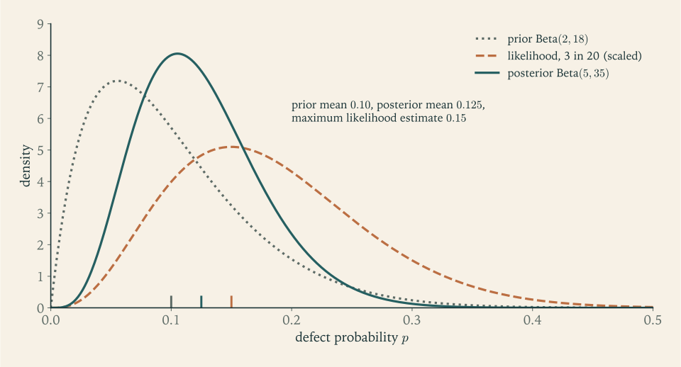
With a uniform prior, \(\operatorname{Beta}(1,1)\) , the same data give the posterior \(\operatorname{Beta}(4,18)\) , with mean \(4/22\approx0.182\) , mode \(3/20=0.15\) (the MLE), and \(95\%\) interval \((0.054,\ 0.363)\) ; the probability that \(p\) exceeds \(0.10\) is then \(0.848\) . Two analysts with different priors reach different posteriors from the same data. That dependence is the most criticised feature of the Bayesian approach and also its most candid one: the assumptions are in plain view, and Section 11.6 examines how much they matter.
11.2 Conjugate families and the weighted-average form
In Example 11.1 the prior and the posterior belonged to the same family, which made the update a matter of adding exponents. A family of priors with this property for a given likelihood is called conjugate.
Proposition 11.2 (three conjugate updates). (a) If \(X\mid p\sim\operatorname{Binomial}(n,p)\) and \(p\sim\operatorname{Beta}(a,b)\) , then \(p\mid x\sim\operatorname{Beta}(a+x,\ b+n-x)\) .
(b) If \(X_1,\dots,X_n\mid\lambda\) are independent \(\operatorname{Poisson}(\lambda)\) and \(\lambda\sim\operatorname{Gamma}(a,b)\) , then \(\lambda\mid x\sim\operatorname{Gamma}\bigl(a+\sum x_i,\ b+n\bigr)\) .
(c) If \(X_1,\dots,X_n\mid\mu\) are independent \(N(\mu,\sigma^2)\) with \(\sigma^2\) known and \(\mu\sim N(\mu_0,\tau^2)\) , then \(\mu\mid x\) is normal with
Proof. (a) \(\pi(p\mid x)\propto p^{a-1}(1-p)^{b-1}\cdot p^x(1-p)^{n-x}=p^{a+x-1}(1-p)^{b+n-x-1}\) .
(b) \(\pi(\lambda\mid x)\propto\lambda^{a-1}e^{-b\lambda}\cdot\lambda^{\sum x_i}e^{-n\lambda}=\lambda^{a+\sum x_i-1}e^{-(b+n)\lambda}\) .
(c) Up to factors free of \(\mu\) , the likelihood is \(\exp\bigl(-\frac{n}{2\sigma^2}(\mu-\bar x)^2\bigr)\) and the prior is \(\exp\bigl(-\frac{1}{2\tau^2}(\mu-\mu_0)^2\bigr)\) . The product is the exponential of a quadratic in \(\mu\) with leading coefficient \(-\frac12\bigl(\frac1{\tau^2}+\frac n{\sigma^2}\bigr)\) and linear coefficient \(\frac{\mu_0}{\tau^2}+\frac{n\bar x}{\sigma^2}\) . Completing the square gives a normal density with precision equal to the leading coefficient times \(-2\) and mean equal to the linear coefficient divided by the precision.
In all three cases the posterior mean is a weighted average of the prior mean and the natural estimate from the data. For the binomial,
so the prior acts like \(a+b\) earlier observations with \(a\) successes. For the Poisson, \(E[\lambda\mid x]=\frac{b}{b+n}\cdot\frac ab+\frac{n}{b+n}\cdot\bar x\) , and the prior acts like \(b\) earlier periods with total count \(a\) . For the normal, the weights are the precisions \(1/\tau^2\) and \(n/\sigma^2\) , the same precision weighting that Exercise 4.2 showed to be optimal for combining independent unbiased estimates. In every case the weight on the data tends to \(1\) as \(n\) grows. The posterior mean is a shrinkage estimator: the data-based estimate pulled toward the prior mean, strongly when data are few and negligibly when they are many.
Example 11.2: A reference length with a design specification
The nine length measurements have \(\bar x=10.1\) , and suppose \(\sigma=0.3\) is known. The part was machined to a nominal \(10.0\) , and the process is known to produce true lengths within about \(\pm0.4\) of nominal; take the prior \(\mu\sim N(10.0,\ 0.2^2)\) . The prior precision is \(1/0.04=25\) and the data precision is \(9/0.09=100\) . The posterior precision is \(125\) , so
The data receive weight \(100/125=0.8\) . The central \(95\%\) posterior interval is \(10.08\pm1.960(0.0894)=(9.905,\ 10.255)\) , and the posterior probability that the part is longer than nominal is \(P(\mu>10\mid x)=\Phi(0.08/0.0894)\approx0.814\) .
Compare the confidence interval of Example 7.1 with known \(\sigma\) : \((9.904,\ 10.296)\) . The Bayesian interval is shorter and shifted toward \(10.0\) . As the prior becomes vague, \(\tau\to\infty\) , the prior precision tends to zero, the posterior tends to \(N(\bar x,\sigma^2/n)\) , and the \(95\%\) posterior interval becomes numerically identical to the confidence interval. The numbers then agree and the interpretations still differ: one is a probability statement about \(\mu\) given these data, the other a statement about the long-run performance of a procedure.
11.3 From posterior to action
A posterior distribution is a complete description of what is believed about \(\theta\) . To report a single estimate, or to choose an action, a loss function is needed, exactly as in Chapter 4.
Definition 11.3 (posterior expected loss, Bayes rule, Bayes risk). Given a loss \(L(\theta,d)\) , the posterior expected loss of an action \(d\) after observing \(x\) is \(\rho(d\mid x)=\int L(\theta,d)\,\pi(\theta\mid x)\,d\theta\) . A Bayes rule \(\delta_\pi\) assigns to each \(x\) an action minimising \(\rho(d\mid x)\) . The Bayes risk of a decision rule \(\delta\) is the average of its risk function with respect to the prior,
The Bayes risk is the average risk of Definition 4.7 with the weight function interpreted as a prior. The two notions of optimality, minimising the posterior expected loss for the data actually observed and minimising the average risk over all possible data, pick out the same rule.
Theorem 11.4 (Bayes rules minimise Bayes risk). If \(\delta_\pi(x)\) minimises \(\rho(d\mid x)\) for every \(x\) with \(m(x)>0\) , then \(r(\pi,\delta_\pi)\le r(\pi,\delta)\) for every decision rule \(\delta\) .
Proof. Write the Bayes risk as a double integral and exchange the order of integration, which is permitted for a nonnegative integrand by Tonelli’s theorem (math.measure-theory.tonelli-fubini-theorem):
using \(\pi(\theta)f(x\mid\theta)=m(x)\pi(\theta\mid x)\) . The bracket is \(\rho(\delta(x)\mid x)\) , which for each \(x\) is at least \(\rho(\delta_\pi(x)\mid x)\) . Integrating against \(m(x)\ge0\) preserves the inequality.
The theorem reduces a minimisation over functions \(\delta\) to a separate minimisation over numbers \(d\) for each \(x\) . For the standard losses the answer is explicit.
Theorem 11.5 (Bayes estimators for three losses). Let the posterior distribution of a real parameter \(\theta\) have a density and finite variance.
(a) Under squared error loss \((\theta-d)^2\) , the Bayes estimate is the posterior mean \(E[\theta\mid x]\) .
(b) Under absolute error loss \(\lvert\theta-d\rvert\) , it is a posterior median.
(c) Under the asymmetric linear loss that charges \(c_u(\theta-d)\) when \(d<\theta\) and \(c_o(d-\theta)\) when \(d>\theta\) , with \(c_u,c_o>0\) , it is a posterior quantile of order \(c_u/(c_u+c_o)\) .
Proof. (a) With \(m=E[\theta\mid x]\) , the decomposition of Theorem 4.2 applied to the posterior distribution gives \(E[(\theta-d)^2\mid x]=\operatorname{Var}(\theta\mid x)+(m-d)^2\) , minimised at \(d=m\) .
(c) Let \(g\) and \(G\) be the posterior density and distribution function. The posterior expected loss is
Differentiating, the boundary terms vanish because each integrand is zero at \(\theta=d\) , and
This is nondecreasing in \(d\) , negative when \(G(d)<c_u/(c_u+c_o)\) and positive when \(G(d)\) exceeds that value, so \(\rho\) is minimised where \(G(d)=c_u/(c_u+c_o)\) .
(b) This is the case \(c_u=c_o\) of (c), for which the quantile is the median.
Part (c) says that when underestimating is more costly than overestimating, the best estimate is deliberately high, and by exactly how much. The same result reappears in Chapter 13, where the “posterior” is any forecast distribution.
Example 11.3: Staffing a switchboard
For the five one-minute counts with total \(20\) , take the prior \(\lambda\sim\operatorname{Gamma}(2,1)\) , which has mean \(2\) and is broad. By Proposition 11.2(b) the posterior is \(\operatorname{Gamma}(22,6)\) , with mean \(22/6\approx3.667\) , standard deviation \(\sqrt{22}/6\approx0.782\) , and median \(3.611\) . The posterior mean is the weighted average \(\tfrac56(4)+\tfrac16(2)\) of the sample mean and the prior mean.
The manager must commit staff for a planned call rate \(d\) . If the true rate exceeds the plan, callers wait, at a cost reckoned at \(3\) per unit of shortfall; if the plan exceeds the true rate, staff are idle, at a cost of \(1\) per unit of excess. By Theorem 11.5(c) the Bayes plan is the posterior quantile of order \(3/(3+1)=0.75\) , which for \(\operatorname{Gamma}(22,6)\) is about \(4.159\) . Under squared error loss the report would be \(3.667\) , under absolute error \(3.611\) , and under this asymmetric loss \(4.159\) . One posterior, three losses, three answers: an estimate is a decision, and it depends on what the estimate is for.
11.4 Credible sets, and how they compare with confidence sets
Definition 11.6 (credible set). A set \(C(x)\subseteq\Theta\) is a credible set of level \(1-\alpha\) if its posterior probability is at least \(1-\alpha\) : \(P(\theta\in C(x)\mid x)\ge1-\alpha\) . An equal-tailed credible interval runs between the \(\alpha/2\) and \(1-\alpha/2\) posterior quantiles. A highest posterior density set has the form \(\{\theta:\pi(\theta\mid x)\ge k\}\) and is the shortest credible set of its level.
A credible interval is what the phrase “the parameter lies in this interval with probability \(0.95\) ” correctly describes. The statement is conditional on the observed data and on the prior. A confidence interval makes a different guarantee, unconditional on any prior and averaged over data that might have been observed. Neither implies the other.
It is nevertheless legitimate to ask how a credible interval performs by the frequentist criterion: for a fixed true \(\theta\) , how often does the interval computed from random data contain it? In regular models with large samples the answer is approximately \(1-\alpha\) , because the posterior is approximately normal with mean near the MLE and variance \(1/(nI(\hat\theta))\) , so credible and confidence intervals nearly coincide. For small samples the coverage depends on \(\theta\) and on the prior.
Example 11.4: Frequentist coverage of a credible interval
For \(X\sim\operatorname{Binomial}(20,p)\) with a uniform prior, the equal-tailed \(95\%\) credible interval after observing \(x\) runs between the \(0.025\) and \(0.975\) quantiles of \(\operatorname{Beta}(x+1,\ 21-x)\) ; for \(x=3\) it is \((0.054,\ 0.363)\) . Its coverage at a fixed true \(p\) is the sum of the binomial probabilities of those \(x\) whose interval contains \(p\) :
| True \(p\) | Coverage of the \(95\%\) credible interval |
|---|---|
| \(0.02\) | \(0.940\) |
| \(0.05\) | \(0.925\) |
| \(0.10\) | \(0.957\) |
| \(0.30\) | \(0.975\) |
| \(0.50\) | \(0.959\) |
The coverage is close to \(0.95\) throughout, sometimes a little above and sometimes a little below, and far better than the Wald interval of Example 7.4, although nothing in its construction aimed at coverage. What the credible interval guarantees exactly is its average coverage with respect to the prior: if \(p\) is drawn from the uniform distribution and then \(X\) from the binomial, the interval contains \(p\) with probability exactly \(0.95\) . A confidence interval guarantees at least \(0.95\) at every \(p\) ; a credible interval guarantees \(0.95\) on average over \(p\) .
With the informative \(\operatorname{Beta}(2,18)\) prior of Example 11.1 the picture changes for values of \(p\) that the prior considers implausible. The same calculation gives coverage \(0.998\) at a true \(p=0.10\) , where the prior is centred, \(0.762\) at \(p=0.30\) , and only \(0.252\) at \(p=0.50\) , because the prior drags the posterior toward small values. That is the appropriate behaviour if the prior is right and a serious failure if it is wrong.
11.5 Bayes rules judged by risk
Chapter 4 ended with a difficulty: risk functions cross, admissibility alone is too weak, and the two reductions of a risk function to a number, its maximum and its average, were stated without a way to find the optimal estimator. Bayes rules resolve this, and they do so on frequentist terms.
Theorem 11.7 (Bayes rules are admissible). Let \(\Theta\) be an interval, let the prior density \(\pi\) be positive on \(\Theta\) , and suppose every estimator has a risk function continuous in \(\theta\) . If \(\delta_\pi\) is a Bayes rule with finite Bayes risk, then \(\delta_\pi\) is admissible.
Proof. Suppose some \(\delta'\) dominated \(\delta_\pi\) : \(R(\theta,\delta')\le R(\theta,\delta_\pi)\) for all \(\theta\) , with strict inequality at some \(\theta^\ast\) . By continuity of the two risk functions the strict inequality holds on an interval around \(\theta^\ast\) , and the prior assigns that interval positive probability. Integrating against \(\pi\) ,
which contradicts Theorem 11.4, according to which \(\delta_\pi\) has the smallest Bayes risk.
Theorem 11.8 (a constant-risk Bayes rule is minimax). If \(\delta_\pi\) is a Bayes rule for some prior \(\pi\) and \(R(\theta,\delta_\pi)\le r(\pi,\delta_\pi)\) for every \(\theta\) , in particular if its risk function is constant, then \(\delta_\pi\) is minimax.
Proof. Let \(\delta'\) be any decision rule. A maximum is at least an average, the average risk of \(\delta'\) is at least that of the Bayes rule, and by hypothesis the Bayes risk bounds the risk of \(\delta_\pi\) everywhere:
So no rule has a smaller maximum risk than \(\delta_\pi\) .
A prior satisfying the hypothesis of Theorem 11.8 is called least favourable: by the chain of inequalities in the proof, no other prior has a larger minimal Bayes risk, so it is the distribution of \(\theta\) that makes the statistician’s task hardest.
Example 11.5: The three analysts of Chapter 4, explained
Let \(X\sim\operatorname{Binomial}(n,p)\) with prior \(\operatorname{Beta}(a,a)\) and squared error loss. The Bayes estimator is the posterior mean \((X+a)/(n+2a)\) , and by the calculation of Example 4.4 its risk is
Uniform prior, \(a=1\) . The estimator \((X+1)/(n+2)\) is Bayes, so by Theorem 11.4 it minimises the uniform-average risk among all estimators, which is the claim made in Section 4.4; for \(n=16\) that minimal average is \(1/108\) . By Theorem 11.7 it is admissible, since risk functions in the binomial model are polynomials in \(p\) and hence continuous.
Least favourable prior, \(a=\sqrt n/2\) . Then \(n-4a^2=0\) and the risk is the constant \(a^2/(n+2a)^2=n/\bigl(4(n+\sqrt n)^2\bigr)\) . By Theorem 11.8 the estimator \((X+\sqrt n/2)/(n+\sqrt n)\) is minimax. For \(n=16\) it is \((X+2)/20\) with risk \(0.01\) : the third analyst’s estimator is the Bayes rule for the \(\operatorname{Beta}(2,2)\) prior and has the smallest possible worst-case mean squared error.
The observed proportion. \(X/n\) corresponds to \(a=0\) , which is not a proper prior. It is not a Bayes rule for squared error loss with any prior density on \((0,1)\) (Exercise 11 shows why), and the theorems above say nothing about it directly; it is in fact admissible, and it is the Bayes rule for a different, weighted loss (Exercise 7).
The second and third analysts were both optimal, for different priors, and the theory tells each what prior their estimator presupposes. This is the use of Bayesian calculation even for someone who does not interpret the prior as belief: Bayes rules are admissible, and scanning over priors generates good procedures whose frequentist properties can then be examined.
11.6 Prediction, priors, and large samples
Prediction. The uncertainty about a future observation \(Y\) has two sources, the randomness of \(Y\) given the parameter and the uncertainty about the parameter. The Bayesian answer averages the first over the second.
Definition 11.9 (posterior predictive distribution). If \(Y\) is conditionally independent of \(X\) given \(\theta\) , with density \(f(y\mid\theta)\) , the posterior predictive density of \(Y\) given \(X=x\) is
Example 11.6: The next ten items
With posterior \(p\mid x\sim\operatorname{Beta}(5,35)\) from Example 11.1, the probability that the next single item is defective is \(\int p\,\pi(p\mid x)\,dp\) , the posterior mean \(0.125\) . For the number \(Y\) of defectives among the next \(m=10\) items, integrating the binomial mass function against the beta posterior gives the beta-binomial distribution
where \(B\) is the beta function. The probability of no defectives is \(P(Y=0\mid x)\approx0.302\) . Substituting the point estimate \(0.125\) into the binomial formula instead gives \(0.875^{10}\approx0.263\) . The plug-in answer is too low because it treats the estimate as exact. The predictive distribution has the same mean, \(10\times0.125=1.25\) , and a larger variance than the plug-in binomial, and it puts more probability on both extremes, including the favourable extreme \(Y=0\) . Ignoring parameter uncertainty makes forecasts overconfident, a theme taken up in Chapter 13.
Choosing a prior. A prior can encode real information, as in Example 11.1, or it can be chosen to be weak, so that the data dominate. Weak priors are often improper, meaning that they do not integrate to a finite value: for instance \(\pi(\mu)\propto1\) on the whole line. An improper prior is acceptable if the posterior it produces is a proper distribution for every data set, and then the usual calculus applies. The flat prior for a normal mean yields the posterior \(N(\bar x,\sigma^2/n)\) of Example 11.2. A flat prior is flat in one parametrization only: uniform on \(p\) is not uniform on the log-odds. The Jeffreys prior, proportional to \(\sqrt{I(\theta)}\) , is constructed to give the same posterior whichever parametrization is used; for the binomial it is \(\operatorname{Beta}(\tfrac12,\tfrac12)\) .
Whatever the choice, the honest practice is a sensitivity analysis: repeat the calculation under several reasonable priors and report how the conclusions move. In Example 11.1 the posterior probability that \(p>0.10\) was \(0.650\) under the informative prior and \(0.848\) under the uniform one. With twenty observations the prior matters, and a report should say so.
Large samples. As \(n\) grows, the likelihood becomes sharply peaked and overwhelms any prior that is positive and continuous near the true parameter. In regular models the posterior is then approximately normal, centred near the MLE with variance \(1/(nI(\hat\theta))\) . This is the Bernstein–von Mises phenomenon, stated here without proof. It has two consequences. Analysts with different priors are driven to agreement by enough data. And Bayesian credible intervals and the likelihood-based confidence intervals of Chapter 9 agree to first order, so in large samples the practical difference between the two approaches lies in interpretation, not in the numbers.
Common mistake. Reading a confidence interval as a credible interval, or the reverse. “\(\mu\) is in \((9.90,10.30)\) with probability \(0.95\) ” is a posterior statement and requires a prior; it happens to be numerically right for a flat prior on a normal mean. “The method covers the truth \(95\%\) of the time” is a coverage statement and holds for a credible interval only approximately, or on average over the prior.
The posterior, the predictive distribution, and the Bayes rule complete the toolkit for a single analysis of given data. Two questions remain about the data themselves. How should they be collected so that a comparison means what it appears to mean? And how should a forecast, Bayesian or otherwise, be judged once the outcome is known? The last two chapters take these in turn.
Exercises
-
A coin lands heads \(7\) times in \(10\) tosses. With a uniform prior on the probability of heads, find the posterior distribution, its mean, mode, and standard deviation.
Answer
Posterior \(\operatorname{Beta}(8,4)\) . Mean \(8/12\approx0.667\) ; mode \(7/10=0.7\) , the MLE; variance \(\frac{8\cdot4}{12^2\cdot13}\approx0.0171\) , standard deviation \(\approx0.131\) .
-
Prove Proposition 11.2(b) in full, and show that the posterior mean of \(\lambda\) is a weighted average of the prior mean \(a/b\) and the sample mean \(\bar x\) with weights \(b/(b+n)\) and \(n/(b+n)\) .
Solution
The \(\operatorname{Gamma}(a,b)\) prior density is proportional to \(\lambda^{a-1}e^{-b\lambda}\) on \(\lambda>0\) . The likelihood of the Poisson sample is
\[ \prod_{i=1}^n\frac{e^{-\lambda}\lambda^{x_i}}{x_i!}\ \propto\ \lambda^{\sum x_i}e^{-n\lambda}, \]the factorials being free of \(\lambda\) . Multiplying,
\[ \pi(\lambda\mid x)\ \propto\ \lambda^{a-1}e^{-b\lambda}\cdot\lambda^{\sum x_i}e^{-n\lambda}=\lambda^{(a+\sum x_i)-1}e^{-(b+n)\lambda}. \]A density on \((0,\infty)\) proportional to \(\lambda^{A-1}e^{-B\lambda}\) is the \(\operatorname{Gamma}(A,B)\) density, since the normalising constant is determined by the requirement that it integrate to one. Hence \(\lambda\mid x\sim\operatorname{Gamma}(a+\sum x_i,\ b+n)\) . The data enter only through \(\sum x_i\) and \(n\) , as sufficiency requires.
The mean of \(\operatorname{Gamma}(A,B)\) is \(A/B\) , so
\[ E[\lambda\mid x]=\frac{a+\sum x_i}{b+n}=\frac{b}{b+n}\cdot\frac ab+\frac{n}{b+n}\cdot\frac{\sum x_i}{n}, \]which is the weighted average of the prior mean \(a/b\) and the sample mean \(\bar x\) with weights \(b/(b+n)\) and \(n/(b+n)\) . The weights are nonnegative and sum to one. The prior behaves like \(b\) previously observed periods containing \(a\) events in total. As \(n\to\infty\) the weight on \(\bar x\) tends to one, and as \(b\to0\) with \(a\to0\) the posterior mean tends to the MLE \(\bar x\) for every \(n\) .
-
Carry out the completion of the square in the proof of Proposition 11.2(c), and verify the formulas with \(n=1\) , \(\sigma^2=1\) , \(\mu_0=0\) , \(\tau^2=1\) , and \(x=2\) .
Hint
Collect the terms in \(\mu^2\) and in \(\mu\) in the exponent: \(-\frac12\bigl(\frac1{\tau^2}+\frac n{\sigma^2}\bigr)\mu^2+\bigl(\frac{\mu_0}{\tau^2}+\frac{n\bar x}{\sigma^2}\bigr)\mu\) . Writing this as \(-\frac{1}{2\tau_n^2}(\mu-\mu_n)^2\) plus a constant identifies \(\tau_n^2\) and \(\mu_n\) . With the given numbers the posterior is \(N(1,\tfrac12)\) .
-
Show in general that updating a prior with independent data \(x\) and then with independent data \(y\) gives the same posterior as updating once with \((x,y)\) . Illustrate with a uniform prior, a first batch of \(2\) successes in \(5\) trials, and a second batch of \(5\) successes in \(5\) trials.
Solution
Let \(x\) and \(y\) be conditionally independent given \(\theta\) , with densities \(f(x\mid\theta)\) and \(g(y\mid\theta)\) .
Two stages. After \(x\) , the posterior is \(\pi_1(\theta)=\pi(\theta\mid x)\propto\pi(\theta)f(x\mid\theta)\) . Using \(\pi_1\) as the prior for \(y\) , the second posterior is proportional to \(\pi_1(\theta)g(y\mid\theta)\propto\pi(\theta)f(x\mid\theta)g(y\mid\theta)\) .
One stage. By conditional independence the joint sampling density of \((x,y)\) is \(f(x\mid\theta)g(y\mid\theta)\) , so the posterior given both is proportional to \(\pi(\theta)f(x\mid\theta)g(y\mid\theta)\) .
The two expressions are proportional as functions of \(\theta\) , and two densities that are proportional are equal. The normalising constants, which differ along the way, never need to be tracked. The argument relies on the conditional independence of the batches given \(\theta\) ; without it the second-stage likelihood would have to be \(g(y\mid\theta,x)\) .
Illustration. Start with \(\operatorname{Beta}(1,1)\) . The first batch, \(2\) successes and \(3\) failures, gives \(\operatorname{Beta}(1+2,\ 1+3)=\operatorname{Beta}(3,4)\) , with mean \(3/7\approx0.429\) . Using that as the prior, the second batch, \(5\) successes and \(0\) failures, gives \(\operatorname{Beta}(3+5,\ 4+0)=\operatorname{Beta}(8,4)\) , with mean \(2/3\) . Updating once with all the data, \(7\) successes and \(3\) failures, gives \(\operatorname{Beta}(1+7,\ 1+3)=\operatorname{Beta}(8,4)\) directly. The order of the batches does not matter either.
-
Ten lifetimes from \(\operatorname{Exp}(\lambda)\) total \(42.0\) hours. With prior \(\lambda\sim\operatorname{Gamma}(1,2)\) , find the posterior distribution, the posterior mean, and the equal-tailed \(95\%\) credible interval for \(\lambda\) , and compare with the confidence interval of Example 7.3.
Answer
The likelihood is \(\lambda^{10}e^{-42\lambda}\) and the prior is proportional to \(e^{-2\lambda}\) , so the posterior is \(\operatorname{Gamma}(11,44)\) , with mean \(11/44=0.25\) and standard deviation \(\sqrt{11}/44\approx0.075\) . The equal-tailed \(95\%\) credible interval is \((0.125,\ 0.418)\) , against the confidence interval \((0.114,\ 0.407)\) : similar in length and shifted slightly upward, because the prior has mean \(0.5\) .
-
For the posterior \(\operatorname{Beta}(5,35)\) of Example 11.1, give the Bayes estimates of \(p\) under squared error loss and under absolute error loss, and explain why they differ in the direction they do.
Answer
Squared error: the posterior mean \(0.125\) . Absolute error: the posterior median, about \(0.119\) . The \(\operatorname{Beta}(5,35)\) density is skewed to the right, and for a right-skewed distribution the mean exceeds the median; squared error penalises the long right tail more heavily and moves the estimate toward it.
-
For \(X\sim\operatorname{Binomial}(n,p)\) with a uniform prior and the weighted loss \(L(p,d)=(d-p)^2/\bigl(p(1-p)\bigr)\) , show that the Bayes estimate is \(x/n\) when \(0<x<n\) .
Solution
For a loss of the form \(w(p)(d-p)^2\) with a positive weight \(w\) , the posterior expected loss is
\[ \rho(d)=\int w(p)(d-p)^2\pi(p\mid x)\,dp=d^2E[w\mid x]-2d\,E[w\,p\mid x]+E[w\,p^2\mid x], \]a quadratic in \(d\) minimised at
\[ d^\ast=\frac{E[w(p)\,p\mid x]}{E[w(p)\mid x]}, \]provided both expectations are finite. Equivalently, \(d^\ast\) is the mean of the distribution with density proportional to \(w(p)\pi(p\mid x)\) .
Here the prior is uniform, so \(\pi(p\mid x)\propto p^x(1-p)^{n-x}\) , and \(w(p)=1/(p(1-p))\) . Then
\[ w(p)\,\pi(p\mid x)\ \propto\ p^{x-1}(1-p)^{n-x-1}, \]which for \(0<x<n\) is the kernel of the \(\operatorname{Beta}(x,\ n-x)\) density, a proper distribution. Its mean is \(x/(x+n-x)=x/n\) . Hence the Bayes estimate is \(d^\ast=x/n\) .
So the observed proportion is a Bayes rule after all, for a loss that penalises errors more heavily when \(p\) is near \(0\) or \(1\) , where the binomial variance is small and a given absolute error is relatively more serious. Under that weighted loss \(X/n\) has constant risk \(E(X/n-p)^2/(p(1-p))=1/n\) , and an extension of Theorem 11.8 shows it is minimax for that loss. The estimator one prefers depends on the loss as well as on the prior. The cases \(x=0\) and \(x=n\) need separate treatment, since the weighted posterior is then not integrable; the limiting values \(0\) and \(1\) are the natural conventions.
-
A colleague states: “A \(95\%\) credible interval contains the true parameter in \(95\%\) of repeated samples.” Using Example 11.4, say exactly what is true and what is false in this statement, and state the sense in which the figure \(95\%\) is guaranteed.
Solution
What is true. A \(95\%\) credible interval \(C(x)\) satisfies \(P(\theta\in C(x)\mid x)=0.95\) : given the data actually observed and the prior, the posterior probability that the parameter lies in the interval is \(0.95\) . Averaging over data, it follows that if \(\theta\) is drawn from the prior and then \(X\) from the model, \(P(\theta\in C(X))=0.95\) exactly. So the figure \(95\%\) is guaranteed as a posterior probability for each data set, and as a frequency over repeated draws of both the parameter and the data.
What is false. The statement refers to repeated samples with the true parameter fixed, which is frequentist coverage. Nothing guarantees that \(P_\theta(\theta\in C(X))=0.95\) for each fixed \(\theta\) . In Example 11.4, with a uniform prior and \(n=20\) , the coverage is \(0.940\) at \(p=0.02\) , \(0.925\) at \(p=0.05\) , \(0.957\) at \(p=0.10\) , and \(0.975\) at \(p=0.30\) . These average to \(0.95\) over the uniform prior, and individually they are above or below it. With the informative \(\operatorname{Beta}(2,18)\) prior the coverage at \(p=0.5\) is only \(0.252\) .
Reconciliation. The colleague’s statement becomes approximately true in large samples for regular models, where posterior and confidence intervals agree to first order, and exactly true in special cases such as the normal mean with a flat prior. In general a credible interval answers “given these data, where is the parameter?” and a confidence interval answers “how often does this procedure succeed?”, and a number attached to one question is not automatically an answer to the other.
-
For a normal sample with known \(\sigma\) , show that the improper prior \(\pi(\mu)\propto1\) gives the posterior \(N(\bar x,\sigma^2/n)\) , and compare the resulting \(95\%\) credible interval with the \(95\%\) confidence interval both numerically and in interpretation.
Solution
With \(\pi(\mu)\propto1\) , the posterior is proportional to the likelihood, which up to factors free of \(\mu\) is \(\exp\bigl(-\frac{n}{2\sigma^2}(\mu-\bar x)^2\bigr)\) , by the identity \(\sum(x_i-\mu)^2=\sum(x_i-\bar x)^2+n(\bar x-\mu)^2\) . As a function of \(\mu\) this is the kernel of the \(N(\bar x,\sigma^2/n)\) density, and it integrates to a finite value, so the posterior is proper: \(\mu\mid x\sim N(\bar x,\sigma^2/n)\) . This is the limit \(\tau\to\infty\) of Proposition 11.2(c).
The equal-tailed \(95\%\) credible interval is \(\bar x\pm1.960\,\sigma/\sqrt n\) , numerically identical to the \(95\%\) confidence interval of Example 7.1. For the nine lengths with \(\sigma=0.3\) , both are \((9.904,\ 10.296)\) .
The interpretations differ. The credible interval says: given the observed \(\bar x=10.1\) and a prior that regards all values of \(\mu\) as equally plausible, the probability that \(\mu\) lies between \(9.904\) and \(10.296\) is \(0.95\) . The confidence interval says: the procedure “report \(\bar X\pm0.196\) ” captures the true \(\mu\) in \(95\%\) of repeated samples, whatever \(\mu\) is; about the particular interval nothing probabilistic is claimed. The coincidence arises because the pivot \(\sqrt n(\bar X-\mu)/\sigma\) is symmetric in \(\bar X\) and \(\mu\) : its distribution is standard normal whether \(\bar X\) is regarded as random with \(\mu\) fixed, or \(\mu\) as random with \(\bar X\) fixed under the flat prior. The agreement is special to location models with flat priors and should not be expected elsewhere.
-
Show that the Jeffreys prior for a Bernoulli probability is \(\operatorname{Beta}(\tfrac12,\tfrac12)\) , and find the posterior mean of \(p\) after \(3\) successes in \(20\) trials under this prior.
Answer
\(I(p)=1/(p(1-p))\) , so \(\sqrt{I(p)}=p^{-1/2}(1-p)^{-1/2}\) , the kernel of \(\operatorname{Beta}(\tfrac12,\tfrac12)\) . The posterior after \(3\) successes in \(20\) is \(\operatorname{Beta}(3.5,\ 17.5)\) , with mean \(3.5/21\approx0.167\) .
-
Let \(\delta(X)=E[\theta\mid X]\) be the Bayes estimator under squared error loss for a proper prior, with finite second moments. Prove that if \(\delta\) is also unbiased, \(E[\delta(X)\mid\theta]=\theta\) for all \(\theta\) , then its Bayes risk is zero.
Hint
Expand the Bayes risk as \(E(\delta-\theta)^2=E\,\delta^2-2E[\delta\theta]+E\,\theta^2\) , with expectations over both \(\theta\) and \(X\) . Conditioning on \(X\) and using \(\delta=E[\theta\mid X]\) gives \(E[\delta\theta]=E\,\delta^2\) . Conditioning on \(\theta\) and using unbiasedness gives \(E[\delta\theta]=E\,\theta^2\) . Substitute both.
-
For a single Bernoulli observation, show that the estimator of Exercise 4.12 with values \((1/4,3/4)\) is the Bayes rule under squared error for the prior \(\operatorname{Beta}(\tfrac12,\tfrac12)\) , and deduce that it is minimax.
Solution
With one Bernoulli observation and prior \(\operatorname{Beta}(\tfrac12,\tfrac12)\) , Proposition 11.2(a) gives the posterior \(\operatorname{Beta}(\tfrac12+x,\ \tfrac32-x)\) , whose mean is
\[ E[p\mid x]=\frac{x+\tfrac12}{2}. \]For \(x=0\) this is \(1/4\) and for \(x=1\) it is \(3/4\) . By Theorem 11.5(a) the posterior mean is the Bayes estimate under squared error loss, so the estimator with values \((\delta(0),\delta(1))=(1/4,3/4)\) is the Bayes rule for this prior. It is the case \(n=1\) , \(a=\sqrt n/2=\tfrac12\) of Example 11.5.
Its risk was computed in Exercise 4.12:
\[ R(p)=(1-p)\bigl(\tfrac14-p\bigr)^2+p\bigl(\tfrac34-p\bigr)^2=\tfrac1{16}\qquad\text{for every }p, \]which also follows from the general formula \(a^2/(n+2a)^2=(1/4)/4\) . The risk is constant, so it equals the Bayes risk \(r(\pi,\delta_\pi)=1/16\) , and the hypothesis \(R(p,\delta_\pi)\le r(\pi,\delta_\pi)\) of Theorem 11.8 holds with equality. Therefore the estimator is minimax: no estimator of \(p\) based on one Bernoulli observation has maximum mean squared error below \(1/16\) . The obvious estimator \(\delta(x)=x\) has maximum risk \(1/4\) , four times as large, attained at \(p=1/2\) ; it does better only for \(p\) near \(0\) or \(1\) . The prior \(\operatorname{Beta}(\tfrac12,\tfrac12)\) is least favourable, putting weight on all values of \(p\) in the way that makes estimation hardest.
-
Use Theorem 11.7 to show that \((X+1)/(n+2)\) is an admissible estimator of a binomial proportion under squared error loss, and explain why the theorem cannot be applied in the same way to \(X/n\) .
Hint
The uniform prior is positive on \((0,1)\) , risk functions are polynomials in \(p\) and so continuous, and the Bayes risk is finite; Theorem 11.7 applies. \(X/n\) would correspond to \(a=b=0\) , for which \(p^{-1}(1-p)^{-1}\) is not integrable: there is no proper prior, no Bayes risk to compare, and the proof has nothing to contradict.
-
With the posterior \(\operatorname{Gamma}(22,6)\) of Example 11.3, derive the posterior predictive probability that the next one-minute count is zero, and compare it with the plug-in value based on the posterior mean, with the MLE of Example 5.4, and with the UMVUE of Example 6.2.
Solution
Given \(\lambda\) , the next count \(Y\) is zero with probability \(e^{-\lambda}\) . The predictive probability is the posterior expectation of that quantity:
\[ P(Y=0\mid x)=E\bigl[e^{-\lambda}\mid x\bigr]=\int_0^\infty e^{-\lambda}\,\frac{b^a}{\Gamma(a)}\lambda^{a-1}e^{-b\lambda}\,d\lambda=\frac{b^a}{(b+1)^a}=\Bigl(\frac{b}{b+1}\Bigr)^a , \]for a \(\operatorname{Gamma}(a,b)\) posterior, because the integrand is a \(\operatorname{Gamma}(a,b+1)\) kernel. With \(a=22\) and \(b=6\) ,
\[ P(Y=0\mid x)=\Bigl(\frac67\Bigr)^{22}\approx0.0337 . \]Four estimates of the probability of an empty minute are now on the table for the same five counts:
- posterior predictive, \((6/7)^{22}\approx0.0337\) ;
- plug-in at the posterior mean, \(e^{-22/6}\approx0.0256\) ;
- maximum likelihood, \(e^{-4}\approx0.0183\) ;
- UMVUE, \(0.8^{20}\approx0.0115\) .
The predictive value exceeds the plug-in value because \(e^{-\lambda}\) is convex: averaging it over the posterior gives more than evaluating it at the posterior mean. It exceeds the MLE for that reason and because the prior, with mean \(2\) , pulls the rate downward. The UMVUE is lowest because unbiasedness for a convex target requires correcting the plug-in estimate downward. The spread, a factor of three between the largest and smallest, shows how little five observations say about a tail probability, and that the criterion chosen matters most when data are scarce.
-
For the posterior \(\operatorname{Beta}(5,35)\) , compute the posterior probability of the hypothesis \(H_0:p\le0.10\) , and compare it with the p-value of the test of \(H_0\) that rejects for large \(X\) when \(x=3\) , \(n=20\) . Explain why the two numbers answer different questions.
Answer
\(P(p\le0.10\mid x)=P(\operatorname{Beta}(5,35)\le0.10)\approx0.350\) . The p-value is \(P_{0.1}(X\ge3)\approx0.323\) . The first is the probability of the hypothesis given the data and the prior; the second is the probability, assuming the boundary value \(p=0.1\) , of data at least as extreme as those seen. Their numerical closeness here is a coincidence of this prior; under the uniform prior the posterior probability is \(0.152\) .
-
For \(3\) successes in \(20\) trials and then for \(30\) successes in \(200\) trials, compute the posterior mean of \(p\) under the priors \(\operatorname{Beta}(1,1)\) , \(\operatorname{Beta}(2,18)\) , and \(\operatorname{Beta}(20,180)\) , and describe what the six numbers show.
Answer
For \(3\) in \(20\) : \(0.182\) , \(0.125\) , \(0.105\) . For \(30\) in \(200\) : \(0.153\) , \(0.145\) , \(0.125\) . With little data the prior dominates and the three analysts disagree widely; with ten times the data all three have moved toward the sample proportion \(0.15\) , and only the prior worth \(200\) observations still pulls noticeably.
-
Show that the variance of the \(\operatorname{Beta}(a+x,\ b+n-x)\) posterior is approximately \(\hat p(1-\hat p)/n\) when \(n\) is large compared with \(a+b\) , and relate this to Theorem 9.6.
Hint
The variance of \(\operatorname{Beta}(A,B)\) is \(AB/\bigl((A+B)^2(A+B+1)\bigr)\) . With \(A=a+x\) and \(B=b+n-x\) , divide numerator and denominator by \(n^3\) and let \(n\to\infty\) with \(x/n=\hat p\) . The limit \(\hat p(1-\hat p)/n\) is \(1/(nI(\hat p))\) , the asymptotic variance of the MLE.
-
Let \(T\) be a sufficient statistic. Prove that the posterior density given the full data \(x\) depends on \(x\) only through \(T(x)\) , for every prior.
Solution
By the factorization theorem (Theorem 3.2), \(f(x\mid\theta)=g(T(x),\theta)\,h(x)\) for functions \(g\) and \(h\) , with \(h\) free of \(\theta\) . For any prior \(\pi\) ,
\[ \pi(\theta\mid x)=\frac{\pi(\theta)\,g(T(x),\theta)\,h(x)}{\int\pi(\theta')\,g(T(x),\theta')\,h(x)\,d\theta'}=\frac{\pi(\theta)\,g(T(x),\theta)}{\int\pi(\theta')\,g(T(x),\theta')\,d\theta'}, \]since \(h(x)\) does not involve the variable of integration and cancels, for every \(x\) with \(h(x)>0\) . The right side depends on \(x\) only through \(T(x)\) . Hence two data sets with the same value of the sufficient statistic lead to the same posterior, whatever the prior.
The converse also holds and gives a Bayesian characterisation of sufficiency: a statistic \(T\) is sufficient exactly when, for every prior, the posterior given \(x\) equals the posterior given \(T(x)\) . The practical content is that Bayesian updating may be carried out on the reduced data. In Example 11.1 only the count of defectives was used, never the order in which they were found; in Proposition 11.2 each posterior depends on the sample through \(\sum x_i\) or \(\bar x\) alone. The agreement with Chapter 3 is not an accident: both the posterior and the frequentist procedures built on the likelihood respond to the data only through the likelihood function, and the sufficient statistic indexes the possible likelihood functions.
-
A lot is accepted or rejected. Accepting a lot with defect rate \(p\) costs \(100p\) ; rejecting it costs \(12\) regardless of \(p\) . Find the Bayes decision as a function of the posterior, and apply it under the prior \(\operatorname{Beta}(2,18)\) when \(3\) defectives are found in \(20\) and when \(2\) are found in \(20\) .
Solution
There are two actions. The loss of accepting is \(100p\) and the loss of rejecting is \(12\) . The posterior expected losses are
\[ \rho(\text{accept}\mid x)=100\,E[p\mid x],\qquad\rho(\text{reject}\mid x)=12 . \]By Definition 11.3 the Bayes decision chooses the smaller: accept when \(100\,E[p\mid x]<12\) , that is, when the posterior mean defect rate is below \(0.12\) , and reject when it is above. Because the loss of accepting is linear in \(p\) , only the posterior mean matters; no other feature of the posterior enters.
Three defectives in twenty. The posterior is \(\operatorname{Beta}(5,35)\) with mean \(0.125\) . The expected loss of accepting is \(12.5\) , which exceeds \(12\) : reject the lot.
Two defectives in twenty. The posterior is \(\operatorname{Beta}(4,36)\) with mean \(0.100\) . The expected loss of accepting is \(10.0\) , below \(12\) : accept the lot.
With this prior the rule can be written directly in terms of the data: the posterior mean is \((2+x)/40\) , which is below \(0.12\) exactly when \(x<2.8\) , so the lot is accepted when at most two defectives are found. The Bayes rule is thus an ordinary acceptance-sampling plan with acceptance number \(2\) , and its frequentist operating characteristic, the probability of acceptance as a function of the true \(p\) , can be computed from the binomial distribution and examined on its own terms. The decision in the first case is close: \(12.5\) against \(12\) . A slightly different prior or cost would reverse it, which a sensitivity analysis would reveal.