A survey of \(200\) customers finds \(60\) who would buy a new product. The analyst wants an interval for the odds of buying, \(p/(1-p)\) , because the pricing model is written in terms of log-odds. Chapter 7 offers nothing directly. The count is binomial, the log-odds is a nonlinear function of the proportion, and no pivot with a tabulated distribution involves it.

Situations like this are the rule. The exact sampling theory of Chapters 2, 7, and 8 covers normal samples, a few other families, and a few statistics in each. For everything else the working tools are approximations that become accurate as the sample grows. This chapter develops them from two imported limit theorems and a first-order Taylor expansion. It answers four questions. When does an estimator converge to the truth? What is its approximate distribution once it does, and how does that distribution transform under a smooth function? Why is the maximum likelihood estimator approximately normal with the smallest possible variance? And how do those facts turn into tests and intervals that need no exact pivot?

An approximation is only as good as its error, and a limit theorem does not come with an error bound. The chapter therefore also pays attention to the cases in which the approximations are poor or simply false.

9.1 Two modes of convergence

Two notions of convergence for random variables are used throughout. Their theory belongs to probability; here are the definitions and the facts that will be needed (math.measure-theoretic-probability.modes-of-convergence).

A sequence \(Y_n\) converges in probability to a constant \(c\) , written \(Y_n\xrightarrow{p}c\) , if \(P(\lvert Y_n-c\rvert>\varepsilon)\to0\) for every \(\varepsilon>0\) . A sequence \(Y_n\) converges in distribution to a random variable \(Y\) , written \(Y_n\xrightarrow{d}Y\) , if \(P(Y_n\le y)\to P(Y\le y)\) at every \(y\) where the distribution function of \(Y\) is continuous. The first says the values of \(Y_n\) concentrate at \(c\) . The second says only that probabilities computed from \(Y_n\) approach those computed from \(Y\) .

The Weak Law of Large Numbers. If \(X_1,X_2,\dots\) are independent and identically distributed with finite mean \(\mu\) , then \(\bar X_n\xrightarrow{p}\mu\) (math.probability-theory.weak-law-large-numbers).

The continuous mapping property. If \(Y_n\xrightarrow{p}c\) and \(g\) is continuous at \(c\) , then \(g(Y_n)\xrightarrow{p}g(c)\) ; if \(Y_n\xrightarrow{d}Y\) and \(g\) is continuous, then \(g(Y_n)\xrightarrow{d}g(Y)\) .

Slutsky’s theorem. If \(Y_n\xrightarrow{d}Y\) and \(A_n\xrightarrow{p}a\) , \(B_n\xrightarrow{p}b\) for constants \(a\) and \(b\) , then \(A_nY_n+B_n\xrightarrow{d}aY+b\) .

Constant limits. Convergence in distribution to a constant is the same as convergence in probability to that constant. The continuous mapping property and the Weak Law hold equally for vectors of fixed dimension, for instance for a pair of sample moments.

Together with the Central Limit Theorem of Section 2.5, these are the whole toolkit. Slutsky’s theorem is what allows an unknown constant in a limit distribution to be replaced by a consistent estimate without changing the limit, which is the step that turns limit theorems into usable procedures.

9.2 Consistency

Definition 1.8 called a sequence of estimators \(T_n\) consistent for \(g(\theta)\) when \(T_n\xrightarrow{p}g(\theta)\) under every \(P_\theta\) . Two general routes establish it.

By (b) and the Weak Law, every method-of-moments estimator that is a continuous function of sample moments is consistent: sample moments converge to population moments, and the estimator is a continuous function of them. The sample variance is consistent for \(\sigma^2\) whenever the variance is finite, and \(S\) is consistent for \(\sigma\) , even though \(S\) is biased for every \(n\) . Consistency and unbiasedness are unrelated properties: \(X_1\) alone is unbiased for \(\mu\) and not consistent, while \(\bar X+1/n\) is biased and consistent.

9.3 Asymptotic normality and the delta method

Consistency says where an estimator ends up. For inference one needs the shape of its fluctuations on the way.

Informally, \(T_n\) is approximately \(N(\theta,v(\theta)/n)\) for large \(n\) . The Central Limit Theorem says that \(\bar X\) is asymptotically normal with asymptotic variance \(\sigma^2\) . An asymptotically normal estimator is consistent (Exercise 17). The next theorem transfers asymptotic normality through smooth functions, and it is the most frequently used result of the chapter.

The theorem says that a smooth function of an approximately normal estimator is approximately normal, with standard error multiplied by \(\lvert g'(\theta)\rvert\) . Near \(\theta\) the function \(g\) is nearly its tangent line, and a linear function of a normal variable is normal; the content of the proof is that the curvature contributes nothing in the limit. When \(g'(\theta)=0\) the limit is degenerate and the theorem gives no useful approximation; a second-order expansion is then needed (Exercise 9).

9.4 Why maximum likelihood works

Chapter 5 left open why maximising the likelihood should produce a good estimator. The answer has two parts: the likelihood is, on average, largest at the true parameter, and near its maximum the log-likelihood is a parabola whose curvature is the Fisher information.

The quantity \(E_{\theta_0}\log\bigl(f(X;\theta_0)/f(X;\theta)\bigr)\) is the Kullback–Leibler divergence from the true distribution to the candidate; the lemma says it is positive unless the candidate is the truth. By the Weak Law, \(\frac1n\ell_n(\theta)=\frac1n\sum\log f(X_i;\theta)\) converges in probability to \(E_{\theta_0}\log f(X;\theta)\) for each fixed \(\theta\) . So for large \(n\) the log-likelihood at any wrong \(\theta\) lies below its value at \(\theta_0\) , with high probability. When there are finitely many candidates this already proves consistency.

For a continuous parameter space the same idea works, but the convergence of \(\frac1n\ell_n(\theta)\) must hold uniformly in \(\theta\) , not just at each point, and that requires extra conditions: for instance a compact parameter space with a log-density that is continuous in \(\theta\) and bounded by an integrable function, or a concave log-likelihood as in exponential families. Under such conditions the MLE is consistent. The proofs are longer and are not given here; in what follows consistency is assumed, and the distribution of the estimator is derived.

The asymptotic variance \(1/I(\theta_0)\) is the Cramér–Rao bound of Theorem 6.2 for one observation. In large samples the MLE has, approximately, the smallest variance that any unbiased estimator can have; such an estimator is called asymptotically efficient. This is the sense in which maximum likelihood is the right default in regular models, and it explains the observation at the end of Chapter 6 that MLEs and UMVUEs tend to be close.

Combined with the delta method and the invariance of Theorem 5.3, the result extends to functions of the parameter: \(\sqrt n(g(\hat\theta_n)-g(\theta_0))\xrightarrow{d}N(0,g'(\theta_0)^2/I(\theta_0))\) . In practice the unknown \(I(\theta_0)\) is replaced by \(I(\hat\theta_n)\) or by the observed information per observation, which is legitimate by Slutsky’s theorem when \(I\) is continuous, and the approximate standard error of \(\hat\theta_n\) is \(1/\sqrt{nI(\hat\theta_n)}\) , as announced in Section 5.4.

Example 9.4: The rate of an exponential distribution

For a random sample from \(\operatorname{Exp}(\lambda)\) the MLE is \(\hat\lambda=1/\bar X\) and \(I(\lambda)=1/\lambda^2\) , so Theorem 9.6 gives \(\sqrt n(\hat\lambda-\lambda)\xrightarrow{d}N(0,\lambda^2)\) . The delta method applied to \(g(m)=1/m\) at \(m=1/\lambda\) , with \(\sqrt n(\bar X-1/\lambda)\xrightarrow{d}N(0,1/\lambda^2)\) and \(g'(m)^2=\lambda^4\) , gives the same limit. Two routes, one answer.

Suppose \(n=50\) lifetimes have mean \(\bar x=2.0\) . Then \(\hat\lambda=0.5\) with standard error \(\hat\lambda/\sqrt n=0.5/\sqrt{50}\approx0.0707\) , and the approximate \(95\%\) interval is

\[ 0.5\pm1.960(0.0707)=(0.361,\ 0.639). \]

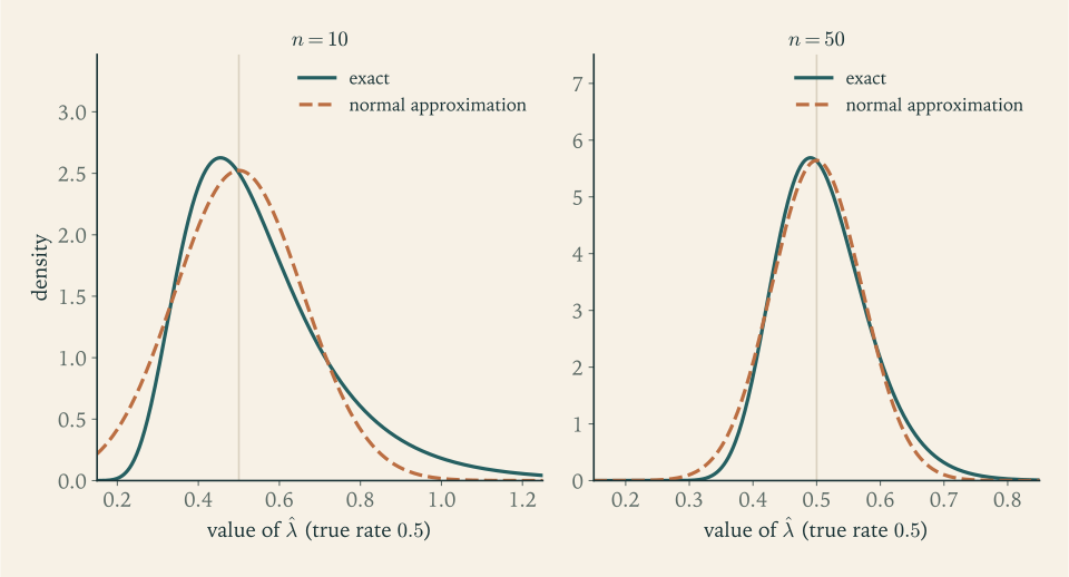
This model has an exact pivot, so the approximation can be checked. Since \(2\lambda\sum X_i\sim\chi^2_{100}\) , whose \(2.5\%\) points are \(74.22\) and \(129.56\) , and \(\sum x_i=100\) , the exact interval is \((74.22/200,\ 129.56/200)=(0.371,\ 0.648)\) . The two agree to about \(0.01\) . The exact interval is shifted to the right because the sampling distribution of \(\hat\lambda\) is skewed to the right, which a normal approximation centred at \(\hat\lambda\) cannot represent. Figure 9.1 shows the exact density of \(\hat\lambda\) and its normal approximation: at \(n=10\) the skewness is plain and the approximation puts visible probability on values the estimator almost never takes, and at \(n=50\) the two nearly coincide.

9.5 Three large-sample tests and the intervals they give

Theorem 9.6 supplies an approximate pivot, and with it tests of \(H_0:\theta=\theta_0\) in any regular model. There are three classical ways to measure the disagreement between the data and \(\theta_0\) , corresponding to three ways of looking at the log-likelihood: the horizontal distance from its peak to \(\theta_0\) , its slope at \(\theta_0\) , and the vertical drop from its peak to its value at \(\theta_0\) .

Each test rejects at approximate level \(\alpha\) when its statistic exceeds \(\chi^2_{1,\alpha}\) ; for \(\alpha=0.05\) the cutoff is \(3.841=1.960^2\) . The three statistics are asymptotically equivalent under \(H_0\) , and they differ in finite samples. The Wald statistic needs only the unrestricted estimate; the score statistic needs only the null value and requires no maximisation; the likelihood ratio needs both and is invariant under reparametrization, which the Wald statistic is not. For a parameter of dimension \(k\) with \(r\) of its components fixed by \(H_0\) , the likelihood ratio statistic \(-2\log\Lambda_n\) converges to \(\chi^2_r\) ; this generalisation, known as Wilks’ theorem, is stated here without proof and is used in Chapter 10.

9.6 When the approximations fail

Each theorem of this chapter has hypotheses, and each hypothesis can fail in practice.

Moving support. Theorem 9.6 requires a regular model. For the uniform distribution on \((0,\theta)\) the MLE converges at rate \(n\) to a non-normal limit (Example 9.1), and applying the normal approximation with a formal “information” is simply wrong.

Boundary parameters. The theorem requires \(\theta_0\) to be an interior point. In the model \(N(\mu,1)\) with \(\mu\ge0\) and true value \(\mu_0=0\) , the MLE is \(\max(\bar X,0)\) , which equals \(0\) with probability \(1/2\) for every \(n\) ; its limiting distribution is half a point mass at zero and half a half-normal, and \(-2\log\Lambda_n\) is not approximately \(\chi^2_1\) .

Zero derivative. The delta method requires \(g'(\theta)\ne0\) for a non-degenerate limit.

Small samples and skewness. A limit theorem gives no error bound. Example 7.4 showed nominal \(95\%\) intervals with \(64\%\) coverage; Figure 9.1 shows how skewness distorts the approximation at \(n=10\) . The quality of the approximation depends on the parametrization, and a transformation that makes the log-likelihood more nearly quadratic, as in Examples 9.2 and 9.3, usually improves it.

Many parameters. The theory fixes the number of parameters and lets \(n\) grow. When the number of parameters is a substantial fraction of the number of observations, the approximations can be seriously off, and the MLE can even be inconsistent.

The remedy in each case is to check. Where an exact distribution is available, compare with it, as in Example 9.4. Where it is not, simulate: generate many samples from the fitted model, apply the procedure to each, and see whether the claimed coverage or level is achieved. A procedure that has not been checked at the sample size in hand is an assumption.

The methods of this chapter treat one parameter in a simple sampling model. The most widely used statistical model has many parameters and observations that are not identically distributed, and remarkably it admits an exact theory. That is the linear model, and it is next.

Exercises

1. Let \(Y_n\) equal \(n\) with probability \(1/n\) and \(0\) otherwise. Show that \(Y_n\xrightarrow{p}0\) although \(E\,Y_n=1\) for every \(n\) and \(E\,Y_n^2\to\infty\) , and explain what this shows about the converse of Theorem 9.1(a).

   Solution

   For any \(\varepsilon\) with \(0<\varepsilon<1\) and any \(n\ge1\) , the event \(\lvert Y_n\rvert>\varepsilon\) is the event \(Y_n=n\) , so

   \[ P(\lvert Y_n-0\rvert>\varepsilon)=\frac1n\longrightarrow0 , \]

   and for \(\varepsilon\ge1\) the probability is at most \(1/n\) as well. Hence \(Y_n\xrightarrow{p}0\) . On the other hand

   \[ E\,Y_n=n\cdot\frac1n=1,\qquad E\,Y_n^2=n^2\cdot\frac1n=n\longrightarrow\infty . \]

   As an estimator of \(0\) , \(Y_n\) is consistent, yet its bias is \(1\) for every \(n\) and its mean squared error grows without bound. So the converse of Theorem 9.1(a) is false: mean squared error tending to zero is sufficient for consistency and not necessary.

   The reason is that convergence in probability concerns where most of the probability lies, while expectations are sensitive to rare, large values. Here an event of vanishing probability \(1/n\) carries a value \(n\) large enough to keep the mean fixed. Consistency says the estimator is close to the target with high probability; it does not control how bad the rare misses are. When the estimators are uniformly bounded this cannot happen, and the two notions agree.

2. Prove that the sample variance \(S_n^2\) is a consistent estimator of \(\sigma^2\) for a random sample from any distribution with finite variance, using the Weak Law and the continuous mapping property and not assuming a finite fourth moment.

   Solution

   Write the sample variance as

   \[ S_n^2=\frac{n}{n-1}\Bigl[\frac1n\sum_{i=1}^nX_i^2-\bar X_n^2\Bigr]. \]

   The variables \(X_i^2\) are independent and identically distributed with finite mean \(E\,X^2=\sigma^2+\mu^2\) , since the variance is finite. By the Weak Law applied to them, \(\frac1n\sum X_i^2\xrightarrow{p}\sigma^2+\mu^2\) . By the Weak Law applied to the \(X_i\) , \(\bar X_n\xrightarrow{p}\mu\) , and by the continuous mapping property with \(g(t)=t^2\) , \(\bar X_n^2\xrightarrow{p}\mu^2\) .

   A difference of two sequences converging in probability converges to the difference of the limits: if each is within \(\varepsilon/2\) of its limit, the difference is within \(\varepsilon\) of the difference of limits, and the probability that either fails tends to zero. So the bracket converges in probability to \(\sigma^2+\mu^2-\mu^2=\sigma^2\) . Finally \(n/(n-1)\to1\) , and multiplying by a deterministic sequence tending to \(1\) does not change the limit. Hence \(S_n^2\xrightarrow{p}\sigma^2\) .

   Only a finite second moment was used. Route (a) of Theorem 9.1 would require the variance of \(S_n^2\) , which involves the fourth moment; route (b) avoids it. By one more application of the continuous mapping property, \(S_n\xrightarrow{p}\sigma\) .

3. For the uniform maximum of Example 9.1, find the smallest sample size for which the probability that \(M_n\) falls short of \(\theta\) by more than \(1\%\) of \(\theta\) is at most \(0.05\) .

   Answer

   \(P(\theta-M_n>0.01\theta)=0.99^n\le0.05\) requires \(n\ge\log0.05/\log0.99\approx298.1\) , so \(n=299\) .

4. Explain why the method-of-moments estimators \(\tilde a=\bar X^2/V\) and \(\tilde b=\bar X/V\) of Example 4.2, where \(V\) is the variance with divisor \(n\) , are consistent for the gamma shape and rate.

   Hint

   By the Weak Law, \(\bar X\xrightarrow{p}a/b\) and \(\frac1n\sum X_i^2\xrightarrow{p}a/b^2+a^2/b^2\) , so \(V\xrightarrow{p}a/b^2\) . The maps \((m,v)\mapsto m^2/v\) and \((m,v)\mapsto m/v\) are continuous wherever \(v>0\) ; apply the continuous mapping property.

5. For a Poisson sample, use the delta method to find the asymptotic distribution of the MLE \(e^{-\bar X}\) of \(e^{-\lambda}\) , compare its asymptotic variance with the Cramér–Rao bound of Section 6.1, and compare the approximation at \(\lambda=4\) , \(n=5\) with the exact variance \(0.00066\) of \(e^{-\bar X}\) .

   Solution

   By the Central Limit Theorem, \(\sqrt n(\bar X-\lambda)\xrightarrow{d}N(0,\lambda)\) . With \(g(t)=e^{-t}\) and \(g'(\lambda)=-e^{-\lambda}\) , Theorem 9.3 gives

   \[ \sqrt n\bigl(e^{-\bar X}-e^{-\lambda}\bigr)\xrightarrow{d}N\bigl(0,\ \lambda e^{-2\lambda}\bigr). \]

   So for large \(n\) the MLE is approximately normal with mean \(e^{-\lambda}\) and variance \(\lambda e^{-2\lambda}/n\) . That is exactly the Cramér–Rao bound for unbiased estimators of \(e^{-\lambda}\) computed in Section 6.1: the MLE is asymptotically efficient, as Theorem 9.6 with the delta method predicts.

   At \(\lambda=4\) and \(n=5\) the approximation gives \(4e^{-8}/5\approx0.00027\) . The exact variance is \(0.00066\) , about two and a half times larger, and by Exercise 6.18 the estimator also has a bias of \(0.0083\) , which the first-order approximation says is zero. With five observations the standard deviation of \(\bar X\) is \(\sqrt{4/5}\approx0.89\) , and over a range of that width the function \(e^{-t}\) is far from linear: it changes by a factor of about \(e^{0.89}\approx2.4\) in each direction. The delta method linearises \(g\) over the region where the estimator is likely to fall, and it is accurate only when that region is small compared with the scale on which \(g\) curves. Here it is not, and the approximation should not be trusted until \(n\) is several times larger.

6. Use the delta method to find the asymptotic distribution of \(1/\bar X\) for a random sample from a distribution with mean \(\mu\ne0\) and variance \(\sigma^2\) , and specialise to the exponential distribution.

   Answer

   With \(g(m)=1/m\) , \(g'(\mu)=-1/\mu^2\) : \(\sqrt n(1/\bar X-1/\mu)\xrightarrow{d}N(0,\sigma^2/\mu^4)\) . For \(\operatorname{Exp}(\lambda)\) , \(\mu=1/\lambda\) and \(\sigma^2=1/\lambda^2\) , giving \(N(0,\lambda^2)\) , as in Example 9.4.

7. For a normal sample, \(\sqrt n(S^2-\sigma^2)\xrightarrow{d}N(0,2\sigma^4)\) . Find the asymptotic distribution of \(\log S^2\) , use it to build an approximate \(95\%\) interval for \(\sigma^2\) from the nine lengths with \(s^2=0.0925\) (taking \(n-1=8\) in place of \(n\) ), and compare with the exact interval of Example 7.2.

   Solution

   With \(g(v)=\log v\) and \(g'(\sigma^2)=1/\sigma^2\) , the delta method gives

   \[ \sqrt n\bigl(\log S^2-\log\sigma^2\bigr)\xrightarrow{d}N\Bigl(0,\ \frac{2\sigma^4}{\sigma^4}\Bigr)=N(0,2). \]

   The logarithm is a variance-stabilising transformation for \(S^2\) : on the log scale the asymptotic variance does not involve \(\sigma^2\) , so \(\sqrt{n/2}(\log S^2-\log\sigma^2)\) is an approximate pivot.

   For the nine lengths, \(\log0.0925\approx-2.381\) , and with \(8\) in place of \(n\) the standard error is \(\sqrt{2/8}=0.5\) . The approximate \(95\%\) interval for \(\log\sigma^2\) is \(-2.381\pm1.960(0.5)=-2.381\pm0.980\) , and exponentiating,

   \[ \bigl(0.0925\,e^{-0.980},\ 0.0925\,e^{0.980}\bigr)\approx(0.0347,\ 0.2465). \]

   The exact interval from Example 7.2 is \((0.0422,\ 0.3395)\) . The approximation is noticeably off: its lower limit is too low and its upper limit is much too low. With \(8\) degrees of freedom the distribution of \(\log S^2\) is still skewed to the left, and the symmetric normal interval on the log scale misplaces both ends. The log transformation removes the dependence of the variance on \(\sigma^2\) , which is necessary for a pivot, but it does not make the distribution normal at this sample size. When an exact pivot exists, it should be used.

8. Find a variance-stabilising transformation for the binomial proportion \(\hat p\) , and state the resulting approximate pivot.

   Hint

   Solve \(g'(p)^2\,p(1-p)=\text{constant}\) : \(g'(p)\propto1/\sqrt{p(1-p)}\) , whose antiderivative is \(2\arcsin\sqrt p\) up to a constant. Then \(2\sqrt n\bigl(\arcsin\sqrt{\hat p}-\arcsin\sqrt p\bigr)\) is approximately standard normal.

9. Let \(\bar X\) be the mean of a random sample with mean \(\mu\) and variance \(\sigma^2\) . (a) Find the limiting distribution of \(n\bar X^2\) when \(\mu=0\) . (b) For Bernoulli data with \(p=1/2\) , find the limiting distribution of \(n\bigl(\hat p(1-\hat p)-\tfrac14\bigr)\) . In both cases explain why Theorem 9.3 gives no useful answer.

   Solution

   (a) When \(\mu=0\) , the Central Limit Theorem gives \(\sqrt n\,\bar X\xrightarrow{d}N(0,\sigma^2)\) . The map \(t\mapsto t^2\) is continuous, so by the continuous mapping property

   \[ n\bar X^2=\bigl(\sqrt n\,\bar X\bigr)^2\xrightarrow{d}\sigma^2\chi^2_1 , \]

   the distribution of the square of a \(N(0,\sigma^2)\) variable. Theorem 9.3 with \(g(t)=t^2\) has \(g'(0)=0\) and says only that \(\sqrt n\,\bar X^2\xrightarrow{d}0\) , which is true and uninformative: the error is of order \(1/n\) , not \(1/\sqrt n\) , and its limit is not normal.

   (b) With \(g(p)=p(1-p)\) , \(g'(p)=1-2p\) vanishes at \(p=1/2\) . Use the exact identity

   \[ \hat p(1-\hat p)-\tfrac14=-\bigl(\hat p-\tfrac12\bigr)^2 . \]

   At \(p=1/2\) , \(\sqrt n(\hat p-\tfrac12)\xrightarrow{d}N(0,\tfrac14)\) , so

   \[ n\Bigl(\hat p(1-\hat p)-\tfrac14\Bigr)=-\Bigl(\sqrt n\bigl(\hat p-\tfrac12\bigr)\Bigr)^2\xrightarrow{d}-\tfrac14\chi^2_1 . \]

   The limit is concentrated on the negative half-line: when \(p=1/2\) the estimator \(\hat p(1-\hat p)\) can only undershoot the true value \(1/4\) , since \(1/4\) is the maximum of the function.

   In both parts the first derivative is zero at the true parameter, so the linear term of the Taylor expansion vanishes and the quadratic term governs. The scaling changes from \(\sqrt n\) to \(n\) and the limit from normal to a multiple of chi-square. A normal-theory interval for \(p(1-p)\) built from the first-order delta method is therefore unreliable when \(p\) is near \(1/2\) .

10. Compute the Kullback–Leibler divergence \(E_{\theta_0}\log\bigl(f(X;\theta_0)/f(X;\theta)\bigr)\) for the family \(N(\theta,1)\) and for the Bernoulli family, and verify in each case that it is zero only when \(\theta=\theta_0\) .

    Answer

    Normal: \(E_{\theta_0}\bigl[\tfrac12(X-\theta)^2-\tfrac12(X-\theta_0)^2\bigr]=\tfrac12(\theta-\theta_0)^2\) . Bernoulli: \(p_0\log\frac{p_0}{p}+(1-p_0)\log\frac{1-p_0}{1-p}\) . Each is nonnegative and vanishes only at \(\theta=\theta_0\) ; for the Bernoulli case this follows from Lemma 9.4 or from minimising over \(p\) .

11. A random sample of size \(100\) from the geometric distribution of Exercise 5.1 has mean \(\bar x=3\) . Give the MLE of \(p\) , its approximate standard error from the Fisher information of Exercise 5.10, and an approximate \(95\%\) confidence interval.

    Answer

    \(\hat p=1/(1+\bar x)=0.25\) . \(I(p)=1/(p^2(1-p))\) , so the standard error is \(\sqrt{\hat p^2(1-\hat p)/n}=\sqrt{0.0625\times0.75/100}\approx0.0217\) , and the interval is \(0.25\pm1.960(0.0217)=(0.208,\ 0.292)\) .

12. A student applies Theorem 9.6 to the uniform distribution on \((0,\theta)\) , computing “\(I(\theta)=1/\theta^2\) ” and concluding that \(\sqrt n(M_n-\theta)\) is approximately \(N(0,\theta^2)\) . State which hypotheses fail, what the correct limiting behaviour is, and how badly the proposed \(95\%\) interval \(M_n\pm1.96\,M_n/\sqrt n\) performs.

    Solution

    Failed hypotheses. Theorem 9.6 requires a regular model. The support \((0,\theta)\) depends on the parameter, so Definition 5.5 fails; the score \(-1/\theta\) does not have mean zero (Exercise 5.12), so \(1/\theta^2\) is not a Fisher information; and the MLE \(M_n\) does not satisfy the likelihood equation, since it sits at a discontinuity of the likelihood (Example 5.3). None of the three ingredients of the proof, a mean-zero score obeying the Central Limit Theorem, an average curvature converging to the information, a stationary point, is available.

    Correct behaviour. By Example 9.1, \(n(\theta-M_n)/\theta\xrightarrow{d}\operatorname{Exp}(1)\) . The error is of order \(1/n\) , always negative, and exponentially distributed in the limit. On the \(\sqrt n\) scale, \(\sqrt n(M_n-\theta)\xrightarrow{p}0\) : the proposed normal limit with variance \(\theta^2\) is not approached at all.

    The proposed interval. Since \(M_n\le\theta\) always, the interval \(M_n\pm1.96M_n/\sqrt n\) covers \(\theta\) exactly when \(\theta\le M_n(1+1.96/\sqrt n)\) , an event of probability

    \[ 1-\Bigl(1+\frac{1.96}{\sqrt n}\Bigr)^{-n}, \]

    by the distribution function \(u^n\) of \(M_n/\theta\) . For \(n=25\) this is \(1-1.392^{-25}\approx0.9997\) . The interval is not too short but absurdly wide: its length is \(2\times1.96M_n/\sqrt n=0.784M_n\) , while the exact \(95\%\) interval \([M_n,\ M_n\,0.05^{-1/25}]\) of Example 7.3 has length \(0.127M_n\) . Half of the proposed interval lies below \(M_n\) , where \(\theta\) cannot be. A method that claims \(95\%\) , delivers \(99.97\%\) , and is six times too long has not understood the model.

13. For a Poisson sample, derive the Wald, score, and likelihood ratio statistics for \(H_0:\lambda=\lambda_0\) , and evaluate all three for \(n=40\) , \(\bar x=4\) , \(\lambda_0=3.5\) .

    Solution

    The log-likelihood is \(\ell(\lambda)=n\bar x\log\lambda-n\lambda\) up to a constant, with \(\ell'(\lambda)=n(\bar x-\lambda)/\lambda\) , \(\hat\lambda=\bar x\) , and \(I(\lambda)=1/\lambda\) .

    Wald. \(W=nI(\hat\lambda)(\hat\lambda-\lambda_0)^2=\dfrac{n(\bar x-\lambda_0)^2}{\bar x}\) .

    Score. \(S=\dfrac{\ell'(\lambda_0)^2}{nI(\lambda_0)}=\dfrac{n^2(\bar x-\lambda_0)^2/\lambda_0^2}{n/\lambda_0}=\dfrac{n(\bar x-\lambda_0)^2}{\lambda_0}\) .

    Likelihood ratio. \(G=2[\ell(\bar x)-\ell(\lambda_0)]=2n\Bigl[\bar x\log\dfrac{\bar x}{\lambda_0}-(\bar x-\lambda_0)\Bigr]\) .

    The Wald and score statistics are the squared standardised difference with the variance \(\lambda/n\) of \(\bar X\) evaluated at the estimate and at the null value respectively.

    For \(n=40\) , \(\bar x=4\) , \(\lambda_0=3.5\) : \(n(\bar x-\lambda_0)^2=40\times0.25=10\) , so

    \[ W=\frac{10}{4}=2.500,\qquad S=\frac{10}{3.5}\approx2.857,\qquad G=80\bigl[4\log(4/3.5)-0.5\bigr]\approx80(0.5341-0.5)=2.730 . \]

    All three are below \(\chi^2_{1,0.05}=3.841\) ; none rejects \(\lambda=3.5\) at the \(5\%\) level. Here \(S>G>W\) because the null value is below the estimate and the Poisson variance increases with \(\lambda\) : the score statistic divides by the smaller variance. The ordering would reverse for a null value above the estimate.

14. Derive the Wilson interval for a binomial proportion by solving the inequality that defines non-rejection by the score test, and evaluate it for \(x=3\) , \(n=20\) at the \(95\%\) level.

    Solution

    The score test does not reject \(p_0\) at level \(\alpha\) when \(n(\hat p-p_0)^2\le z^2p_0(1-p_0)\) , with \(z=z_{\alpha/2}\) . Expanding and collecting powers of \(p_0\) ,

    \[ (n+z^2)\,p_0^2-(2n\hat p+z^2)\,p_0+n\hat p^2\le0 . \]

    The left side is an upward parabola in \(p_0\) , so the inequality holds between its two roots. The discriminant is

    \[ (2n\hat p+z^2)^2-4(n+z^2)n\hat p^2=4n\hat pz^2+z^4-4z^2n\hat p^2=z^2\bigl(4n\hat p(1-\hat p)+z^2\bigr), \]

    and the roots are

    \[ p_0=\frac{2n\hat p+z^2\pm z\sqrt{4n\hat p(1-\hat p)+z^2}}{2(n+z^2)}=\frac{\hat p+\dfrac{z^2}{2n}\pm z\sqrt{\dfrac{\hat p(1-\hat p)}{n}+\dfrac{z^2}{4n^2}}}{1+\dfrac{z^2}{n}}, \]

    after dividing numerator and denominator by \(2n\) . This is the Wilson interval.

    For \(x=3\) , \(n=20\) , \(z=1.960\) : \(z^2=3.8415\) , \(z^2/n=0.1921\) , \(z^2/(2n)=0.0960\) , and \(z^2/(4n^2)=0.0024\) . The centre is \((0.15+0.0960)/1.1921\approx0.2064\) and the half-width is \(1.960\sqrt{0.006375+0.0024}/1.1921\approx0.1540\) . The interval is \((0.052,\ 0.360)\) .

    Compared with the Wald interval \((-0.006,0.306)\) , the centre has moved from \(0.15\) toward \(1/2\) and both endpoints are inside \((0,1)\) . Compared with the Clopper–Pearson interval \((0.032,0.379)\) it is a little narrower, which is the source of its coverage being close to, and occasionally slightly below, the nominal level.

15. For the switchboard data of Example 5.1, find the set of \(\lambda\) not rejected by the likelihood ratio test at approximate level \(0.05\) , and explain its relation to the relative-likelihood cutoff \(0.15\) used in that example.

    Answer

    \(G(\lambda)\le3.841\) is equivalent to relative likelihood \(L(\lambda)/L(\hat\lambda)\ge e^{-3.841/2}\approx0.1465\) . For the switchboard data the set is approximately \((2.49,\ 6.02)\) . The cutoff \(0.15\) of Example 5.1 is this value rounded: a relative-likelihood interval at level \(0.15\) is an approximate \(95\%\) confidence interval.

16. Using the Wald interval for a Poisson mean, find the number of observation periods needed for the \(95\%\) interval to have half-width about \(10\%\) of \(\lambda\) when \(\lambda\) is about \(4\) .

    Answer

    \(1.960\sqrt{\lambda/n}\le0.1\lambda\) requires \(n\ge1.960^2/(0.01\lambda)\approx96.0\) at \(\lambda=4\) , so about \(97\) periods.

17. Prove that if \(\sqrt n(T_n-\theta)\xrightarrow{d}N(0,v)\) then \(T_n\xrightarrow{p}\theta\) , directly from the definitions and without Slutsky’s theorem.

    Solution

    Fix \(\varepsilon>0\) and \(\eta>0\) ; we must show \(P(\lvert T_n-\theta\rvert>\varepsilon)<\eta\) for all large \(n\) . Let \(Y_n=\sqrt n(T_n-\theta)\) and let \(Y\sim N(0,v)\) . If \(v=0\) the limit is the constant \(0\) ; otherwise \(Y\) has a continuous distribution. In either case choose \(K>0\) so large that \(P(\lvert Y\rvert\ge K)<\eta/2\) , and such that \(K\) and \(-K\) are continuity points of the distribution function of \(Y\) .

    Convergence in distribution gives \(P(Y_n\le K)\to P(Y\le K)\) and \(P(Y_n\le-K)\to P(Y\le-K)\) , hence

    \[ P(\lvert Y_n\rvert>K)\le1-P(Y_n\le K)+P(Y_n\le-K)\longrightarrow P(Y>K)+P(Y\le-K)<\frac\eta2 . \]

    So there is \(n_1\) with \(P(\lvert Y_n\rvert>K)<\eta\) for all \(n\ge n_1\) .

    Now \(\lvert T_n-\theta\rvert>\varepsilon\) is the event \(\lvert Y_n\rvert>\varepsilon\sqrt n\) . For \(n\ge(K/\varepsilon)^2\) we have \(\varepsilon\sqrt n\ge K\) , so this event is contained in \(\lvert Y_n\rvert>K\) . Therefore, for \(n\ge\max\{n_1,(K/\varepsilon)^2\}\) ,

    \[ P(\lvert T_n-\theta\rvert>\varepsilon)\le P(\lvert Y_n\rvert>K)<\eta . \]

    Since \(\varepsilon\) and \(\eta\) were arbitrary, \(T_n\xrightarrow{p}\theta\) . The idea is that a sequence converging in distribution is bounded in probability, and dividing a bounded sequence by \(\sqrt n\) sends it to zero.

18. For Poisson data, compare two estimators of \(e^{-\lambda}\) : the proportion of zero counts and the MLE \(e^{-\bar X}\) . Find the ratio of their asymptotic variances as a function of \(\lambda\) , and evaluate it at \(\lambda=0.5\) and \(\lambda=4\) .

    Solution

    Proportion of zeros. Let \(Q_n=\frac1n\sum\mathbf 1\{X_i=0\}\) . It is a sample mean of Bernoulli variables with success probability \(e^{-\lambda}\) , so \(\sqrt n(Q_n-e^{-\lambda})\xrightarrow{d}N\bigl(0,\ e^{-\lambda}(1-e^{-\lambda})\bigr)\) .

    MLE. By Exercise 9.5, \(\sqrt n(e^{-\bar X}-e^{-\lambda})\xrightarrow{d}N(0,\lambda e^{-2\lambda})\) .

    Ratio. The asymptotic variance of the MLE divided by that of the proportion is

    \[ \frac{\lambda e^{-2\lambda}}{e^{-\lambda}(1-e^{-\lambda})}=\frac{\lambda e^{-\lambda}}{1-e^{-\lambda}}=\frac{\lambda}{e^{\lambda}-1}. \]

    Since \(e^\lambda-1>\lambda\) for \(\lambda>0\) , the ratio is below \(1\) for every \(\lambda\) : the MLE is asymptotically more precise everywhere. At \(\lambda=0.5\) the ratio is \(0.5/(e^{0.5}-1)\approx0.771\) ; at \(\lambda=4\) it is \(4/(e^4-1)\approx0.075\) .

    The ratio is the asymptotic relative efficiency of the proportion with respect to the MLE: the proportion needs \(1/0.771\approx1.3\) times as many observations to match the MLE when \(\lambda=0.5\) , and about \(13\) times as many when \(\lambda=4\) . When zeros are common the proportion of zeros uses most of the information; when they are rare it throws nearly all of it away, because it ignores whether a nonzero count was \(1\) or \(9\) . The price of the MLE’s efficiency is its reliance on the Poisson form: the proportion of zeros is consistent for \(P(X=0)\) under any distribution, and \(e^{-\bar X}\) is not.

19. For a random sample of size \(n\) from \(\operatorname{Exp}(\lambda)\) , show that the Wald interval \(\hat\lambda\pm1.96\,\hat\lambda/\sqrt n\) covers \(\lambda\) exactly when \(\lambda\sum X_i\) lies in a fixed interval, and use the gamma distribution to compute its exact coverage for \(n=10\) .

    Answer

    With \(c=1.96/\sqrt n\) and \(\hat\lambda=n/\sum X_i\) , the interval contains \(\lambda\) exactly when \(n(1-c)\le\lambda\sum X_i\le n(1+c)\) , and \(\lambda\sum X_i\sim\operatorname{Gamma}(n,1)\) . For \(n=10\) , \(c\approx0.620\) and the coverage is \(P(3.80\le\operatorname{Gamma}(10,1)\le16.20)\approx0.955\) . The total coverage is close to nominal, but the two tail errors are unequal: almost all of the misses are on one side.