An agronomist applies fertiliser to eight plots at rates \(x=1,2,\dots,8\) (in units of ten kilograms per hectare) and records the yields
in tonnes per hectare. Yield rises with fertiliser, roughly along a line, but not exactly: the seventh plot does better than the eighth, and the other steps from one rate to the next range from \(0.2\) to \(2.3\) tonnes. Three questions arise at once. What line best describes the relationship? How precisely do eight plots determine its slope? And what yield should be expected, and with what uncertainty, at a rate of \(5\) , or at a rate of \(12\) that nobody has tried?
So far every model in this book has been a random sample: observations with a common distribution. Here the observations have different means, and the way the mean depends on \(x\) is the object of study. The linear model handles this, and it is the most widely used model in statistics. It is also one of the few multi-parameter models with an exact finite-sample theory, built from the geometry of projections and the orthogonal-invariance lemma of Chapter 2. This chapter develops that theory: least squares, its optimality, exact \(t\) and \(F\) inference, and, because a fitted model is only as good as its assumptions, the examination of residuals.
10.1 The model and three levels of assumption
Definition 10.1 (linear model). A linear model for observations \(y=(y_1,\dots,y_n)^{\top}\) is
where \(X\) is a known \(n\times p\) design matrix, \(\beta\in\mathbb R^p\) is an unknown parameter vector, and \(\varepsilon\) is an unobserved random error vector. The assumptions on \(\varepsilon\) come in three levels:
(A1) \(E\,\varepsilon=0\) , so that \(E\,y=X\beta\) ;
(A2) in addition \(\operatorname{Cov}(\varepsilon)=\sigma^2I_n\) : the errors are uncorrelated with common variance \(\sigma^2\) ;
(A3) in addition \(\varepsilon\sim N(0,\sigma^2I_n)\) : the errors are independent normal variables.
Throughout, \(X\) is assumed to have full column rank \(p\) , with \(p<n\) .
“Linear” refers to the parameters: the mean \(X\beta\) is a linear function of \(\beta\) . The columns of \(X\) may be nonlinear functions of measured quantities. The straight line \(y_i=\beta_0+\beta_1x_i+\varepsilon_i\) has rows \((1,x_i)\) ; the quadratic \(y_i=\beta_0+\beta_1x_i+\beta_2x_i^2+\varepsilon_i\) has rows \((1,x_i,x_i^2)\) and is equally a linear model. A comparison of \(k\) group means is a linear model whose columns are indicators of group membership. The random sample from \(N(\mu,\sigma^2)\) is the case in which \(X\) is a single column of ones.
The design matrix is treated as fixed. If the \(x\) values were themselves random, the analysis is understood conditionally on the values that occurred. The full-rank assumption is the identifiability condition of Chapter 1: the mean vector \(X\beta\) determines \(\beta\) uniquely exactly when the columns of \(X\) are linearly independent, and Exercise 1.15 was an example in which they were not.
Each level of assumption buys a result. (A1) makes least squares unbiased. (A2) makes it the best linear unbiased estimator and gives its variance. (A3) gives exact distributions for tests and intervals. Keeping track of which conclusion needs which assumption shows what is lost when an assumption fails.
10.2 Least squares as projection
The least-squares estimator is the value of \(\beta\) that minimises the sum of squared deviations \(Q(\beta)=\lVert y-X\beta\rVert^2=\sum_i(y_i-x_i^{\top}\beta)^2\) , where \(x_i^{\top}\) is the \(i\) -th row of \(X\) .
Theorem 10.2 (normal equations). If \(X\) has full column rank, then \(X^{\top}X\) is invertible, and \(Q\) has the unique minimiser
which is the unique solution of the normal equations \(X^{\top}X\hat\beta=X^{\top}y\) , equivalently \(X^{\top}(y-X\hat\beta)=0\) .
Proof. If \(X^{\top}Xv=0\) then \(v^{\top}X^{\top}Xv=\lVert Xv\rVert^2=0\) , so \(Xv=0\) , and full column rank gives \(v=0\) . Hence \(X^{\top}X\) is invertible and the normal equations have exactly one solution \(\hat\beta\) . For any \(\beta\) write \(y-X\beta=(y-X\hat\beta)+X(\hat\beta-\beta)\) . The two parts are orthogonal, since \((\hat\beta-\beta)^{\top}X^{\top}(y-X\hat\beta)=0\) by the normal equations. Therefore
with equality only when \(X(\hat\beta-\beta)=0\) , that is, when \(\beta=\hat\beta\) .
The proof is a picture. The set of all vectors \(X\beta\)
is the column space of \(X\)
, a \(p\)
-dimensional subspace of \(\mathbb R^n\)
. Least squares finds the point of that subspace closest to \(y\)
, and the closest point of a subspace is the orthogonal projection (math.linear-algebra.projection-as-best-approximation). The normal equations say that the residual vector \(e=y-X\hat\beta\)
is orthogonal to every column of \(X\)
. The same computation, viewed as fitting an overdetermined system, is treated in Linear Algebra (math.linear-algebra.least-squares-fit).
Definition 10.3 (hat matrix, fitted values, residuals). The hat matrix is \(H=X(X^{\top}X)^{-1}X^{\top}\) . The fitted values are \(\hat y=X\hat\beta=Hy\) and the residuals are \(e=y-\hat y=(I-H)y\) . The residual sum of squares is \(\mathrm{RSS}=\lVert e\rVert^2\) .
\(H\) is the matrix of the orthogonal projection onto the column space of \(X\) . It is symmetric and satisfies \(H^2=H\) , its trace is \(p\) , and \(HX=X\) ; \(I-H\) is the projection onto the orthogonal complement, with trace \(n-p\) . The decomposition \(y=\hat y+e\) splits the data into a part explained by the model and a part orthogonal to everything the model can produce, and \(\lVert y\rVert^2=\lVert\hat y\rVert^2+\lVert e\rVert^2\) .
For the straight line \(y_i=\beta_0+\beta_1x_i+\varepsilon_i\) , solving the two normal equations gives the familiar formulas
Example 10.1: Fitting the fertiliser line
For the eight plots, \(\sum x_i=36\) , \(\sum x_i^2=204\) , \(\sum y_i=44.4\) , and \(\sum x_iy_i=238.8\) . The normal equations are
Equivalently, \(\bar x=4.5\) , \(\bar y=5.55\) , \(S_{xx}=204-8(4.5)^2=42\) , and \(S_{xy}=238.8-8(4.5)(5.55)=39\) , so
Each additional unit of fertiliser is associated with about \(0.93\) tonnes more yield. The fitted values and residuals are
| \(x_i\) | 1 | 2 | 3 | 4 | 5 | 6 | 7 | 8 |
|---|---|---|---|---|---|---|---|---|
| \(y_i\) | \(2.4\) | \(2.6\) | \(4.7\) | \(5.4\) | \(5.9\) | \(6.3\) | \(8.6\) | \(8.5\) |
| \(\hat y_i\) | \(2.300\) | \(3.229\) | \(4.157\) | \(5.086\) | \(6.014\) | \(6.943\) | \(7.871\) | \(8.800\) |
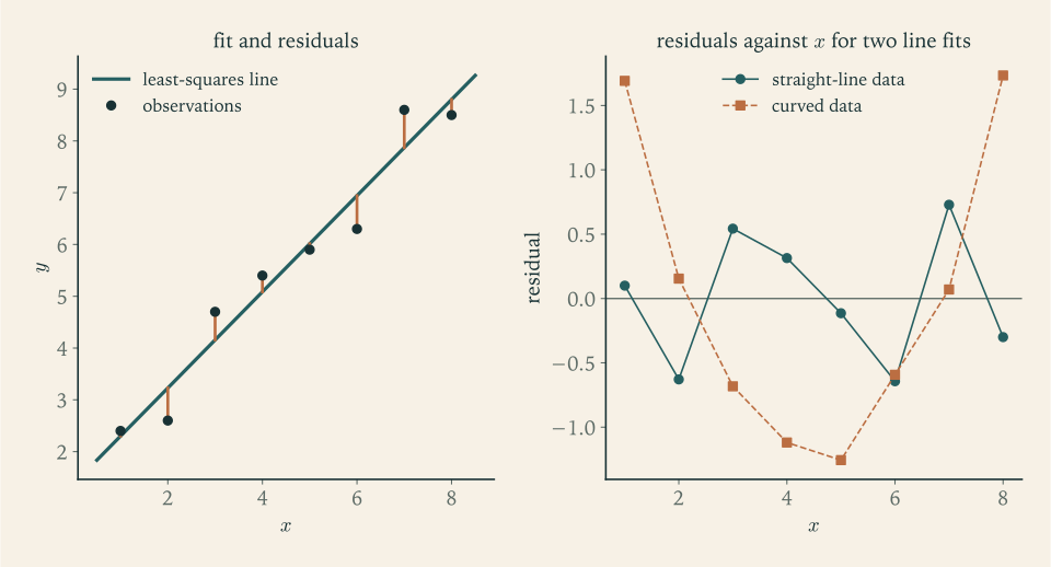
| \(e_i\) | \(0.100\) | \(-0.629\) | \(0.543\) | \(0.314\) | \(-0.114\) | \(-0.643\) | \(0.729\) | \(-0.300\) |
The residuals sum to zero and are orthogonal to the \(x\) column, \(\sum x_ie_i=0\) , as the normal equations require. The residual sum of squares is \(\mathrm{RSS}\approx1.846\) . The total variation of the yields about their mean is \(S_{yy}=\sum(y_i-\bar y)^2=38.06\) , so the line accounts for the fraction \(R^2=1-1.846/38.06\approx0.9515\) of it. The left panel of Figure 10.1 shows the line and the residuals as vertical segments.
10.3 What least squares estimates, and how well
Under the model, \(\hat\beta\) is a random vector, a linear function of \(y\) . Its first two moments need only the first two levels of assumption.
Theorem 10.4 (mean, covariance, and variance estimate). Under (A1), \(E\,\hat\beta=\beta\) . Under (A2), \(\operatorname{Cov}(\hat\beta)=\sigma^2(X^{\top}X)^{-1}\) and \(E\,\mathrm{RSS}=(n-p)\sigma^2\) , so that
is an unbiased estimator of \(\sigma^2\) .
Proof. Substituting \(y=X\beta+\varepsilon\) gives \(\hat\beta=\beta+(X^{\top}X)^{-1}X^{\top}\varepsilon\) . Taking expectations with \(E\,\varepsilon=0\) gives \(E\,\hat\beta=\beta\) . For a constant matrix \(A\) , \(\operatorname{Cov}(A\varepsilon)=A\operatorname{Cov}(\varepsilon)A^{\top}\) ; with \(A=(X^{\top}X)^{-1}X^{\top}\) and \(\operatorname{Cov}(\varepsilon)=\sigma^2I\) this is \(\sigma^2(X^{\top}X)^{-1}X^{\top}X(X^{\top}X)^{-1}=\sigma^2(X^{\top}X)^{-1}\) .
For the residuals, \(e=(I-H)y=(I-H)\varepsilon\) because \((I-H)X=0\) . Since \(I-H\) is symmetric and idempotent, \(\mathrm{RSS}=\varepsilon^{\top}(I-H)\varepsilon=\sum_{i,j}(I-H)_{ij}\varepsilon_i\varepsilon_j\) . Under (A2), \(E\,\varepsilon_i\varepsilon_j\) is \(\sigma^2\) when \(i=j\) and \(0\) otherwise, so \(E\,\mathrm{RSS}=\sigma^2\sum_i(I-H)_{ii}=\sigma^2\operatorname{tr}(I-H)=\sigma^2(n-p)\) .
The divisor \(n-p\) generalises the \(n-1\) of the sample variance: fitting \(p\) parameters uses up \(p\) dimensions of the data, and the residual vector lives in the remaining \(n-p\) . For the straight line the covariance matrix gives
The slope is estimated precisely when \(S_{xx}\) is large, that is, when the \(x\) values are spread out; this is a statement about design, available before any data are collected. The fitted line is most precisely known at \(\bar x\) and progressively less so away from it.
Is there a better estimator than least squares? Among linear unbiased estimators, no.
Theorem 10.5 (Gauss–Markov). Assume (A2), and let \(c\in\mathbb R^p\) . Among all estimators of \(c^{\top}\beta\) that are linear in \(y\) , of the form \(a^{\top}y\) , and unbiased for every \(\beta\) , the least-squares estimator \(c^{\top}\hat\beta\) has the smallest variance.
Proof. The estimator \(a^{\top}y\) has expectation \(a^{\top}X\beta\) , which equals \(c^{\top}\beta\) for every \(\beta\) exactly when \(X^{\top}a=c\) . The least-squares estimator is \(c^{\top}\hat\beta=a_0^{\top}y\) with \(a_0=X(X^{\top}X)^{-1}c\) , and \(X^{\top}a_0=c\) . Let \(a\) be any vector with \(X^{\top}a=c\) and put \(d=a-a_0\) . Then \(X^{\top}d=c-c=0\) , so \(d^{\top}a_0=d^{\top}X(X^{\top}X)^{-1}c=0\) : the vectors \(d\) and \(a_0\) are orthogonal. Under (A2), \(\operatorname{Var}(a^{\top}y)=\sigma^2\lVert a\rVert^2\) , and
with equality only when \(d=0\) . Hence \(\operatorname{Var}(a^{\top}y)\ge\operatorname{Var}(c^{\top}\hat\beta)\) .
Least squares is the best linear unbiased estimator. No normality was used; the theorem needs only uncorrelated errors with equal variances. Both qualifications in the name matter. If the error variances are unequal or the errors are correlated, least squares remains unbiased but is no longer best, and a weighted version takes its place (Exercise 7). And the comparison is with linear estimators only: with heavy-tailed errors, nonlinear estimators can be much better. Under normality the restriction to linear estimators can be dropped, since \((\hat\beta,\mathrm{RSS})\) is then a complete sufficient statistic and \(\hat\beta\) is the UMVUE (Exercise 19).
10.4 Exact inference under normality
With normal errors the distribution of everything computed so far is known exactly.
Theorem 10.6 (distribution theory of the normal linear model). Under (A3),
and \(\hat\beta\) and \(\mathrm{RSS}\) are independent. Consequently, for every \(c\ne0\) ,
Proof. Choose an orthonormal basis \(q_1,\dots,q_p\) of the column space of \(X\) and extend it to an orthonormal basis \(q_1,\dots,q_n\) of \(\mathbb R^n\) . Let \(Q\) be the orthogonal matrix with these columns and put \(W=Q^{\top}\varepsilon/\sigma\) . By Lemma 2.4 the components \(W_1,\dots,W_n\) are independent standard normal variables. In these coordinates the projection \(H\) keeps the first \(p\) components and \(I-H\) keeps the last \(n-p\) :
Therefore \(\mathrm{RSS}=\lVert(I-H)\varepsilon\rVert^2=\sigma^2\sum_{j=p+1}^nW_j^2\) , and \(\mathrm{RSS}/\sigma^2\sim\chi^2_{n-p}\) by Definition 2.3. Next, \(\hat\beta-\beta=(X^{\top}X)^{-1}X^{\top}\varepsilon\) , and since \(X^{\top}=X^{\top}H\) , this equals \((X^{\top}X)^{-1}X^{\top}H\varepsilon\) , a function of \(W_1,\dots,W_p\) only. So \(\hat\beta\) depends on the first \(p\) coordinates and \(\mathrm{RSS}\) on the last \(n-p\) , and they are independent. \(\hat\beta\) is a linear function of the normal vector \(\varepsilon\) , hence normal, with the mean and covariance of Theorem 10.4. Finally, \(c^{\top}\hat\beta-c^{\top}\beta\) is normal with mean \(0\) and variance \(\sigma^2c^{\top}(X^{\top}X)^{-1}c\) ; dividing by its standard deviation gives a standard normal variable independent of \(\mathrm{RSS}/\sigma^2\sim\chi^2_{n-p}\) , and the ratio in the statement is that variable divided by \(\sqrt{(\mathrm{RSS}/\sigma^2)/(n-p)}\) .
Theorem 2.5 is the special case \(p=1\) with \(X\) a column of ones. The \(t\) pivot gives tests and confidence intervals for any linear combination of the coefficients: a single coefficient, a difference of two, or the mean response \(x_0^{\top}\beta\) at a new point. For a new observation \(y_0=x_0^{\top}\beta+\varepsilon_0\) at \(x_0\) , independent of the data, the argument of Proposition 7.6 gives the prediction pivot
Example 10.2: Slope, mean response, and prediction for the fertiliser data
Here \(n-p=6\) , \(\hat\sigma^2=1.846/6\approx0.3076\) , and \(\hat\sigma\approx0.555\) tonnes.
Slope. The standard error is \(\hat\sigma/\sqrt{S_{xx}}=0.555/\sqrt{42}\approx0.0856\) . For \(H_0:\beta_1=0\) ,
on \(6\) degrees of freedom: overwhelming evidence that yield depends on the rate. With \(t_{6,0.025}\approx2.447\) the \(95\%\) interval for the slope is \(0.9286\pm2.447(0.0856)=(0.719,\ 1.138)\) .
Mean yield at \(x_0=5\) . The estimate is \(1.3714+0.9286(5)\approx6.014\) , with standard error \(0.555\sqrt{1/8+0.25/42}\approx0.201\) . The \(95\%\) interval for the mean yield of plots fertilised at rate \(5\) is \(6.014\pm0.491=(5.52,\ 6.51)\) .
A single new plot at \(x_0=5\) . The prediction standard error is \(0.555\sqrt{1+1/8+0.25/42}\approx0.590\) , and the \(95\%\) prediction interval is \(6.014\pm1.443=(4.57,\ 7.46)\) , three times as wide.
Extrapolation to \(x_0=12\) . The estimate is \(12.514\) , and now \((x_0-\bar x)^2/S_{xx}=56.25/42\approx1.34\) dominates: the interval for the mean is \(12.514\pm1.642\) and the prediction interval is \(12.514\pm2.130\) . These are much wider than at \(x_0=5\) , and they are still optimistic, because they assume that the straight line continues to hold four units beyond the largest rate tried. The intervals quantify sampling error under the model. They contain no allowance for the model being wrong outside the range of the data, and with fertiliser it certainly is: yields level off and then fall.
10.5 Comparing nested models
Many questions take the form: does a larger model fit significantly better than a smaller one contained in it? Is a quadratic term needed? Do three varieties differ? Let the smaller model have design matrix \(X_0\) of rank \(p_0\) whose column space is contained in that of \(X\) , of rank \(p>p_0\) , and let \(\mathrm{RSS}_0\) and \(\mathrm{RSS}\) be the two residual sums of squares. Since the larger model minimises over a larger set, \(\mathrm{RSS}\le\mathrm{RSS}_0\) .
Theorem 10.7 (F-test for nested linear models). Under (A3), if the smaller model is true, that is, if \(E\,y\) lies in the column space of \(X_0\) , then
Proof. Choose the orthonormal basis in the proof of Theorem 10.6 so that \(q_1,\dots,q_{p_0}\) span the column space of \(X_0\) and \(q_1,\dots,q_p\) span that of \(X\) . When \(E\,y\) lies in the smaller space, both residual vectors are projections of \(\varepsilon\) alone, and in the coordinates \(W=Q^{\top}\varepsilon/\sigma\) ,
The last two involve disjoint sets of independent standard normal variables, so they are independent, with \((\mathrm{RSS}_0-\mathrm{RSS})/\sigma^2\sim\chi^2_{p-p_0}\) and \(\mathrm{RSS}/\sigma^2\sim\chi^2_{n-p}\) . The ratio of the two, each divided by its degrees of freedom, has the \(F\) distribution by Definition 2.3, and \(\sigma^2\) cancels.
Large values of \(F\) are evidence against the smaller model: the extra parameters reduce the residual sum of squares by more than chance would. When the smaller model is false the numerator is inflated by the squared length of the part of \(E\,y\) that it cannot represent. The \(F\) statistic is a decreasing function of the likelihood ratio statistic \(\Lambda\) of Definition 8.9 (Exercise 12), so rejecting for large \(F\) is rejecting for small \(\Lambda\) : this is the likelihood ratio test with its exact null distribution. When \(p-p_0=1\) it is the square of the \(t\) statistic for the single added coefficient: for the fertiliser line against the constant-mean model, \(F=(38.06-1.846)/(1.846/6)\approx117.7=10.85^2\) .
Example 10.3: Three varieties compared
Twelve plots are sown with three wheat varieties, four plots each, and the yields are
| Variety | Yields | Mean |
|---|---|---|
| A | \(20,\ 22,\ 19,\ 23\) | \(21\) |
| B | \(25,\ 27,\ 24,\ 28\) | \(26\) |
| C | \(22,\ 21,\ 24,\ 21\) | \(22\) |
The larger model gives each variety its own mean (\(p=3\) , with \(X\) made of three indicator columns); the smaller says all twelve plots share one mean (\(p_0=1\) ). In the larger model the least-squares fit of each plot is its variety mean, so
In the smaller model the fit is the grand mean \(23\) , and \(\mathrm{RSS}_0=\sum(y_{ij}-23)^2=82\) . The difference \(\mathrm{RSS}_0-\mathrm{RSS}=56\) equals \(4\bigl[(21-23)^2+(26-23)^2+(22-23)^2\bigr]\) , the variation between the variety means. Then
with p-value \(P(F_{2,9}\ge9.69)\approx0.0057\) ; the \(5\%\) point of \(F_{2,9}\) is \(4.26\) . The varieties differ. This is one-way analysis of variance: a comparison of the variation between group means with the variation within groups. The estimate of \(\sigma^2\) is the within-group mean square \(26/9\approx2.89\) . The \(F\) -test says only that the three means are not all equal; which differ, and by how much, is answered by \(t\) intervals for differences such as \(\mu_B-\mu_A\) , with Bonferroni adjustment if several are examined.
10.6 Criticism: residuals, leverage, and what regression does not show
All of the inference above is conditional on the model. The residuals are the evidence about whether the model is adequate, because they are what remains after the model has explained what it can. Under (A2), \(\operatorname{Cov}(e)=\sigma^2(I-H)\) , so \(\operatorname{Var}(e_i)=\sigma^2(1-h_{ii})\) , where the diagonal element \(h_{ii}\) of the hat matrix is the leverage of observation \(i\) . For the straight line \(h_{ii}=1/n+(x_i-\bar x)^2/S_{xx}\) : points far from \(\bar x\) have high leverage, pull the line toward themselves, and have small residuals for that very reason. Leverages lie between \(0\) and \(1\) and sum to \(p\) .
If the model is right, the residuals should look like noise: no trend against the fitted values or against any explanatory variable, roughly constant spread, no gross outliers. Each kind of pattern points to a specific failure. Curvature in a plot of residuals against \(x\) means the mean function is misspecified, a failure of (A1). A spread that fans out means unequal variances, a failure of (A2). A few very large residuals, or a markedly non-normal shape, bear on (A3).
Example 10.4: A high R-squared and a wrong model
On the same eight \(x\) values suppose the responses are
The least-squares line is \(\hat y=-2.729+2.237x\) , with \(R^2\approx0.957\) , a figure that would often be reported as a good fit. The residuals are
positive at both ends and negative in the middle: the right panel of Figure 10.1 shows the unmistakable U shape next to the patternless residuals of the fertiliser fit. The line is the wrong model. Adding a quadratic term gives a nested comparison: the residual sum of squares falls from \(9.542\) to \(0.0653\) , and
on \((1,5)\) degrees of freedom. A measure of how much variation a model explains does not show whether the model is correct; the residual plot does. Under the straight-line model the estimate \(\hat\sigma^2=9.542/6\) is inflated by the unmodelled curvature, every standard error is wrong, and predictions are biased in a systematic, predictable direction.
A different failure cannot be seen in any residual plot.
Theorem 10.8 (omitted-variable bias). Suppose the true model is \(y=X_1\beta_1+X_2\beta_2+\varepsilon\) with \(E\,\varepsilon=0\) , but \(y\) is regressed on \(X_1\) alone, giving \(\tilde\beta_1=(X_1^{\top}X_1)^{-1}X_1^{\top}y\) . Then
Proof. Substitute the true model: \(\tilde\beta_1=(X_1^{\top}X_1)^{-1}X_1^{\top}(X_1\beta_1+X_2\beta_2+\varepsilon)=\beta_1+(X_1^{\top}X_1)^{-1}X_1^{\top}X_2\beta_2+(X_1^{\top}X_1)^{-1}X_1^{\top}\varepsilon\) , and take expectations.
The bias vanishes when \(\beta_2=0\) , so that the omitted variables do not matter, or when \(X_1^{\top}X_2=0\) , so that they are orthogonal to the included ones. Otherwise the coefficient of an included variable absorbs part of the effect of every omitted variable correlated with it. The matrix \((X_1^{\top}X_1)^{-1}X_1^{\top}X_2\) holds the coefficients from regressing each omitted variable on the included ones.
Example 10.5: A coefficient that changes sign
Six workers have hours of training \(x_1=1,2,3,4,5,6\) and years of experience \(x_2=6,5,5,3,2,1\) ; the experienced workers were given less training. Their output is
generated as \(10+x_1+2x_2\) plus small errors. Regressing \(y\) on both variables gives
close to the generating coefficients: with experience held fixed, each hour of training adds about one unit of output. Regressing \(y\) on training alone gives
a negative slope: output appears to fall with training. Theorem 10.8 accounts for the reversal exactly. The regression of \(x_2\) on \(x_1\) has slope \(-18/17.5\approx-1.0286\) , and to four decimals
Nothing is wrong with the arithmetic of the short regression, and its residuals look unremarkable. It answers a different question: how output varies with training among workers as they come, with their experience varying along with their training. Whether that or the coefficient \(1.088\) is the “effect of training” is not a question the data can settle.
Common mistake. Interpreting a regression coefficient as the change in \(y\) that would result from changing \(x\) . The coefficient describes how the mean of \(y\) differs between units that differ in \(x\) , with the other included variables equal. It describes an intervention only if nothing that affects \(y\) and is correlated with \(x\) has been left out, and no amount of data can verify that from within the regression.
That limitation is the motivation for the last part of this book. Chapter 12 shows how to make the omitted-variable term vanish by construction, by assigning \(x\) at random. Before that, Chapter 11 takes up a different extension: what changes when prior knowledge about \(\beta\) , or about any parameter, is expressed as a probability distribution.
Exercises
-
Write the design matrix for the straight-line model with \(x=(0,1,2,3)\) , compute \(X^{\top}X\) and its inverse, and read off \(\operatorname{Var}\hat\beta_1\) and \(\operatorname{Cov}(\hat\beta_0,\hat\beta_1)\) in terms of \(\sigma^2\) .
Answer
\(X\) has rows \((1,0)\) , \((1,1)\) , \((1,2)\) , \((1,3)\) . \(X^{\top}X=\begin{pmatrix}4&6\\6&14\end{pmatrix}\) with determinant \(20\) and inverse \(\begin{pmatrix}0.7&-0.3\\-0.3&0.2\end{pmatrix}\) . So \(\operatorname{Var}\hat\beta_1=0.2\,\sigma^2\) , which is \(\sigma^2/S_{xx}\) with \(S_{xx}=5\) , and \(\operatorname{Cov}(\hat\beta_0,\hat\beta_1)=-0.3\,\sigma^2\) .
-
For \(x=(0,1,2,3)\) and \(y=(1,3,4,8)\) , compute the least-squares line, the fitted values, the residuals, the residual sum of squares, and \(\hat\sigma^2\) .
Answer
\(\bar x=1.5\) , \(\bar y=4\) , \(S_{xx}=5\) , \(S_{xy}=11\) : \(\hat\beta_1=2.2\) , \(\hat\beta_0=0.7\) . Fitted values \(0.7\) , \(2.9\) , \(5.1\) , \(7.3\) ; residuals \(0.3\) , \(0.1\) , \(-1.1\) , \(0.7\) ; \(\mathrm{RSS}=1.80\) ; \(\hat\sigma^2=1.80/2=0.90\) .
-
Prove that when the model contains an intercept the residuals sum to zero, the mean of the fitted values equals \(\bar y\) , and the fitted line passes through \((\bar x,\bar y)\) in simple regression; and that the residuals are orthogonal to the fitted values in every linear model.
Solution
The normal equations state \(X^{\top}e=0\) : the residual vector is orthogonal to every column of \(X\) .
Residuals sum to zero. If the model contains an intercept, one column of \(X\) is the vector of ones, \(\mathbf 1\) , and orthogonality to it reads \(\mathbf 1^{\top}e=\sum_ie_i=0\) .
Mean of fitted values. Since \(y_i=\hat y_i+e_i\) , summing gives \(\sum y_i=\sum\hat y_i+0\) , so the fitted values have the same mean as the observations, \(\bar y\) .
The line passes through the point of means. In simple regression the fitted value at \(x\) is \(\hat\beta_0+\hat\beta_1x\) . Averaging the fitted values over the data, \(\bar y=\hat\beta_0+\hat\beta_1\bar x\) , which says exactly that the point \((\bar x,\bar y)\) lies on the fitted line.
Residuals orthogonal to fitted values. In any linear model the fitted vector \(\hat y=X\hat\beta\) is a linear combination of the columns of \(X\) , and \(e\) is orthogonal to each column, so
\[ \hat y^{\top}e=\hat\beta^{\top}X^{\top}e=\hat\beta^{\top}0=0 . \]This holds with or without an intercept. It is the Pythagorean relation \(\lVert y\rVert^2=\lVert\hat y\rVert^2+\lVert e\rVert^2\) in another form. A consequence for diagnostics: in a model with an intercept, where the residuals also sum to zero, the residuals and the fitted values have zero sample covariance, so a plot of one against the other has no linear trend whatever is wrong with the model; only nonlinear patterns in such a plot are informative. Without an intercept the first three statements, and with them this consequence, can fail, which is one reason for including an intercept unless there is a specific reason not to.
-
Prove that the hat matrix is symmetric and idempotent with trace \(p\) , that \(0\le h_{ii}\le1\) , and that for the straight-line model \(h_{ii}=1/n+(x_i-\bar x)^2/S_{xx}\) .
Hint
\(H^{\top}=H\) because \((X^{\top}X)^{-1}\) is symmetric; \(H^2=X(X^{\top}X)^{-1}X^{\top}X(X^{\top}X)^{-1}X^{\top}=H\) ; \(\operatorname{tr}H=\operatorname{tr}\bigl((X^{\top}X)^{-1}X^{\top}X\bigr)=\operatorname{tr}I_p\) . From \(H=H^2\) and symmetry, \(h_{ii}=\sum_jh_{ij}^2\ge h_{ii}^2\) . For the line, compute \(x_i^{\top}(X^{\top}X)^{-1}x_i\) with \(x_i=(1,x_i)^{\top}\) , most easily after centring \(x\) .
-
For the straight-line model derive \(\operatorname{Var}\hat\beta_1=\sigma^2/S_{xx}\) and \(\operatorname{Cov}(\hat\beta_0,\hat\beta_1)=-\sigma^2\bar x/S_{xx}\) from \(\sigma^2(X^{\top}X)^{-1}\) , and explain what the first formula implies for choosing the \(x\) values when the range available is fixed.
Solution
For the straight line with rows \((1,x_i)\) ,
\[ X^{\top}X=\begin{pmatrix}n&\sum x_i\\\sum x_i&\sum x_i^2\end{pmatrix},\qquad\det(X^{\top}X)=n\sum x_i^2-\Bigl(\sum x_i\Bigr)^2=n\,S_{xx}, \]because \(S_{xx}=\sum x_i^2-n\bar x^2\) . Inverting the \(2\times2\) matrix,
\[ (X^{\top}X)^{-1}=\frac{1}{nS_{xx}}\begin{pmatrix}\sum x_i^2&-\sum x_i\\-\sum x_i&n\end{pmatrix}. \]By Theorem 10.4, \(\operatorname{Cov}(\hat\beta)=\sigma^2(X^{\top}X)^{-1}\) . Reading off entries,
\[ \operatorname{Var}\hat\beta_1=\sigma^2\frac{n}{nS_{xx}}=\frac{\sigma^2}{S_{xx}},\qquad\operatorname{Cov}(\hat\beta_0,\hat\beta_1)=-\sigma^2\frac{\sum x_i}{nS_{xx}}=-\frac{\sigma^2\bar x}{S_{xx}}. \]The covariance is negative when \(\bar x>0\) : if the slope is overestimated, the line pivots about \((\bar x,\bar y)\) and the intercept is underestimated. Centring the explanatory variable, so that \(\bar x=0\) , makes the two estimates uncorrelated.
Design: for a fixed number of observations the slope variance is minimised by making \(S_{xx}\) as large as possible. If \(x\) is restricted to an interval, \(S_{xx}\) is largest when half the observations are placed at each end. For the fertiliser range \([1,8]\) with eight plots that gives \(S_{xx}=8(3.5)^2=98\) against \(42\) for equal spacing, and a slope variance smaller by the factor \(42/98\approx0.43\) . The price is that a two-point design provides no information about curvature: it is optimal only if the straight-line model is known to hold. Equal spacing sacrifices some precision to keep the model checkable.
-
In the straight-line model with \(x_i=i\) for \(i=1,\dots,8\) , the “endpoint estimator” of the slope is \((y_8-y_1)/7\) . Show that it is linear and unbiased, compute its variance, and compare with the least-squares variance in the light of Theorem 10.5.
Solution
Write the estimator as \(a^{\top}y\) with \(a=(-\tfrac17,0,0,0,0,0,0,\tfrac17)^{\top}\) ; it is linear in \(y\) . Its expectation is
\[ \frac{E\,y_8-E\,y_1}{7}=\frac{(\beta_0+8\beta_1)-(\beta_0+\beta_1)}{7}=\beta_1 \]for every \((\beta_0,\beta_1)\) , so it is unbiased. Under (A2) the two observations are uncorrelated with variance \(\sigma^2\) each, so
\[ \operatorname{Var}\Bigl(\frac{y_8-y_1}{7}\Bigr)=\frac{2\sigma^2}{49}\approx0.0408\,\sigma^2 . \]The least-squares slope has variance \(\sigma^2/S_{xx}=\sigma^2/42\approx0.0238\,\sigma^2\) . The endpoint estimator’s variance is larger by the factor \((2/49)\times42=12/7\approx1.71\) , as the Gauss–Markov theorem guarantees it must be: least squares has the smallest variance in the class of linear unbiased estimators, and the endpoint estimator belongs to that class.
The comparison is instructive because the endpoint estimator uses the two most informative observations and discards the other six. It is not foolish, only inefficient: the six interior points carry the remaining \(42-24.5=17.5\) units of \(S_{xx}\) . In the two-point design of Exercise 10.5, where all observations sit at the ends, the endpoint idea applied to the two group means is least squares.
-
Suppose \(\operatorname{Var}(\varepsilon_i)=\sigma^2/w_i\) with known positive weights \(w_i\) and uncorrelated errors. Find a transformation of the model to which Theorem 10.5 applies, and deduce the form of the best linear unbiased estimator.
Hint
Multiply the \(i\) -th equation by \(\sqrt{w_i}\) : with \(y_i^\ast=\sqrt{w_i}y_i\) and rows \(\sqrt{w_i}x_i^{\top}\) , the transformed errors have common variance \(\sigma^2\) , so Theorem 10.5 applies to the transformed model. Its least-squares estimator minimises \(\sum w_i(y_i-x_i^{\top}\beta)^2\) and equals \((X^{\top}WX)^{-1}X^{\top}Wy\) with \(W=\operatorname{diag}(w_i)\) .
-
Consider the model of Exercise 1.15, in which \(x_{i2}=2x_{i1}\) . Show that \(X^{\top}X\) is singular, that the normal equations have infinitely many solutions, and that all of them give the same fitted values.
Solution
The design matrix has columns \(u=(x_{11},\dots,x_{n1})^{\top}\) and \(2u\) , with \(u\ne0\) . Then
\[ X^{\top}X=\begin{pmatrix}u^{\top}u&2u^{\top}u\\2u^{\top}u&4u^{\top}u\end{pmatrix}=u^{\top}u\begin{pmatrix}1&2\\2&4\end{pmatrix}, \]whose determinant is \((u^{\top}u)^2(4-4)=0\) : it is singular. Equivalently, \(X(2,-1)^{\top}=2u-2u=0\) , so the columns are linearly dependent and \(X\) has rank \(1\) .
The normal equations \(X^{\top}X\beta=X^{\top}y\) read
\[ u^{\top}u\,(\beta_1+2\beta_2)=u^{\top}y\qquad\text{and}\qquad2u^{\top}u\,(\beta_1+2\beta_2)=2u^{\top}y , \]the same equation twice. They are satisfied by every \((\beta_1,\beta_2)\) on the line \(\beta_1+2\beta_2=u^{\top}y/u^{\top}u\) : infinitely many solutions.
For any such solution the fitted vector is \(X\beta=\beta_1u+2\beta_2u=(\beta_1+2\beta_2)u=\dfrac{u^{\top}y}{u^{\top}u}\,u\) , which does not depend on which solution was chosen. It is the orthogonal projection of \(y\) onto the line spanned by \(u\) , and the projection onto a subspace is unique even when the coordinates used to describe it are not. This is Exercise 1.15 seen from the estimation side: the data determine the identifiable combination \(\beta_1+2\beta_2\) and the fitted values, and nothing else.
-
For the data of Exercise 2, test \(H_0:\beta_1=0\) at the \(5\%\) level and give a \(95\%\) confidence interval for the slope.
Answer
Standard error \(\sqrt{0.90/5}\approx0.424\) ; \(t=2.2/0.424\approx5.19\) on \(2\) degrees of freedom, with two-sided p-value \(\approx0.035\) : reject at the \(5\%\) level. With \(t_{2,0.025}\approx4.303\) the interval is \(2.2\pm4.303(0.424)=(0.37,\ 4.03)\) .
-
For the fertiliser data, compute the \(95\%\) confidence interval for the mean yield and the \(95\%\) prediction interval at \(x_0=4.5\) , and compare their widths with those at \(x_0=5\) and \(x_0=12\) in Example 10.2.
Answer
At \(x_0=4.5=\bar x\) the estimate is \(\bar y=5.55\) . Mean: \(5.55\pm2.447\times0.555\sqrt{1/8}=5.55\pm0.480\) , that is, \((5.07,\ 6.03)\) . Prediction: \(5.55\pm2.447\times0.555\sqrt{1+1/8}=5.55\pm1.439\) , that is, \((4.11,\ 6.99)\) . Both are the narrowest available; the half-widths at \(x_0=5\) are \(0.491\) and \(1.443\) , and at \(x_0=12\) they are \(1.642\) and \(2.130\) .
-
For the model \(y_i=\beta x_i+\varepsilon_i\) through the origin, derive the least-squares estimator and its variance under (A2). Show that if the true intercept is zero, fitting an unnecessary intercept increases the variance of the slope estimator, and by what factor.
Solution
Through the origin. The design matrix is the single column \(x\) , so \(X^{\top}X=\sum x_i^2\) and
\[ \hat\beta=\frac{\sum x_iy_i}{\sum x_i^2},\qquad\operatorname{Var}\hat\beta=\frac{\sigma^2}{\sum x_i^2}, \]by Theorems 10.2 and 10.4 with \(p=1\) .
With an unnecessary intercept. If the true intercept is zero, the two-parameter model is still correct, with \(\beta_0=0\) , so the slope estimator \(S_{xy}/S_{xx}\) is unbiased, with variance \(\sigma^2/S_{xx}\) . Since \(S_{xx}=\sum x_i^2-n\bar x^2\le\sum x_i^2\) , its variance is at least as large. The ratio is
\[ \frac{\sigma^2/S_{xx}}{\sigma^2/\sum x_i^2}=\frac{\sum x_i^2}{S_{xx}}=1+\frac{n\bar x^2}{S_{xx}}. \]For the fertiliser design, \(\sum x_i^2=204\) and \(S_{xx}=42\) : the factor is \(204/42\approx4.86\) . Estimating an intercept that is not needed multiplies the slope variance by nearly five here, because the \(x\) values are far from zero relative to their spread.
This is the bias-variance trade of Chapter 4 in a regression setting. The smaller model is far more precise if it is true, and biased if it is false; by Theorem 10.8 forcing the line through the origin when \(\beta_0\ne0\) biases the slope by \(\beta_0\sum x_i/\sum x_i^2\) . The larger model is safe and costly. The choice should rest on subject knowledge about whether the mean response must vanish at \(x=0\) , and it can be checked with a \(t\) -test of \(\beta_0=0\) .
-
Show that in the normal linear model the likelihood ratio statistic for a nested hypothesis satisfies \(\Lambda^{2/n}=\mathrm{RSS}/\mathrm{RSS}_0\) , and deduce that \(\Lambda\) is a decreasing function of the \(F\) statistic of Theorem 10.7.
Hint
For any linear model the maximised normal likelihood is \((2\pi\,\mathrm{RSS}/n)^{-n/2}e^{-n/2}\) , as in Example 8.5. Take the ratio for the two models, then write \(\mathrm{RSS}_0/\mathrm{RSS}=1+\frac{p-p_0}{n-p}F\) .
-
Express the comparison of the two processes in Example 7.5 as a nested linear-model comparison, compute the \(F\) statistic, and verify that it equals the square of the pooled \(t\) statistic of Example 8.4.
Answer
Larger model: separate means, \(\mathrm{RSS}=1.580+1.244=2.824\) on \(16\) degrees of freedom. Smaller model: one common mean; \(\mathrm{RSS}_0-\mathrm{RSS}=\frac{8\times10}{18}(0.81)^2=2.916\) . \(F=2.916/(2.824/16)\approx16.52\) on \((1,16)\) degrees of freedom, and \(4.065^2\approx16.52\) .
-
A report states: “The regression has \(R^2=0.957\) , so the linear model is appropriate and its predictions are reliable.” Using Example 10.4, explain what \(R^2\) does and does not measure and name the check that should have been made.
Solution
\(R^2=1-\mathrm{RSS}/S_{yy}\) is the fraction of the variation of \(y\) about its mean that the fitted model reproduces. It compares the model with one alternative only, the constant-mean model, and says the line does far better than a constant. It does not compare the line with any richer model, so it cannot show that the line is the right form.
In Example 10.4 the response increases steeply and smoothly, so any increasing line captures most of its variation, hence \(R^2=0.957\) . Yet the residuals are positive, then negative for four consecutive points, then positive: the mean function is curved, and the straight line is systematically wrong. A quadratic reduces the residual sum of squares from \(9.542\) to \(0.0653\) , a factor of about \(146\) .
“Predictions are reliable” fails in three ways. Within the range of the data, predictions are biased in a known direction, too low at the ends and too high in the middle. The standard errors are computed from \(\hat\sigma^2=9.542/6\approx1.59\) , which reflects lack of fit and not noise, so intervals are miscalibrated. Outside the range the error grows without bound, since a line and a parabola diverge.
The check that should have been made is a plot of residuals against \(x\) or against fitted values, which shows the U shape at once, followed if desired by a formal \(F\) -test for an added quadratic term. A high \(R^2\) is compatible with a wrong model, and a low \(R^2\) is compatible with a correct one in which the noise is simply large.
-
For the data of Example 10.5, verify the omitted-variable formula numerically: compute the slope of the regression of \(x_2\) on \(x_1\) and show that the short-regression slope equals the long-regression coefficient of \(x_1\) plus that slope times the long-regression coefficient of \(x_2\) . Explain why the identity is exact for the estimates and not only in expectation.
Solution
Regression of \(x_2\) on \(x_1\) : \(\bar x_1=3.5\) , \(\sum(x_{i1}-3.5)^2=17.5\) , and
\[ \sum(x_{i1}-3.5)\,x_{i2}=(-2.5)(6)+(-1.5)(5)+(-0.5)(5)+(0.5)(3)+(1.5)(2)+(2.5)(1)=-18 , \]so the slope is \(-18/17.5\approx-1.0286\) .
Long regression: \(\hat\beta_1\approx1.0884\) and \(\hat\beta_2\approx2.1081\) . Then
\[ \hat\beta_1+(-1.0286)\,\hat\beta_2\approx1.0884-2.1684=-1.0800 , \]which is the short-regression slope \(\tilde\beta_1=-1.0800\) .
Why the identity is exact: let \(\hat y=X_1\hat\beta_1+X_2\hat\beta_2\) and \(e\) be the fitted values and residuals of the long regression, where \(X_1\) contains the intercept column and \(x_1\) . Then \(y=X_1\hat\beta_1+X_2\hat\beta_2+e\) with \(X_1^{\top}e=0\) . Apply the short-regression formula to this expression for \(y\) :
\[ \tilde\beta_1=(X_1^{\top}X_1)^{-1}X_1^{\top}y=\hat\beta_1+(X_1^{\top}X_1)^{-1}X_1^{\top}X_2\,\hat\beta_2+0 . \]This is the algebra of Theorem 10.8 with the estimates in place of the parameters and the residual vector, which is exactly orthogonal to \(X_1\) , in place of the error vector, which is orthogonal only on average. The identity therefore holds in every data set, not just in expectation. Whenever a variable is dropped, the coefficients of the remaining ones change by precisely the dropped coefficient times the regression of the dropped variable on the retained ones.
-
Show that under (A3) the least-squares estimator is the maximum likelihood estimator of \(\beta\) , find the MLE of \(\sigma^2\) , and compute its bias.
Answer
The log-likelihood is \(-\frac n2\log(2\pi\sigma^2)-\lVert y-X\beta\rVert^2/(2\sigma^2)\) ; for every \(\sigma^2\) it is maximised in \(\beta\) by minimising \(\lVert y-X\beta\rVert^2\) , so the MLE of \(\beta\) is \(\hat\beta\) . Then \(\hat\sigma^2_{\mathrm{MLE}}=\mathrm{RSS}/n\) , with expectation \((n-p)\sigma^2/n\) and bias \(-p\sigma^2/n\) .
-
A straight line is fitted to five points with \(x=(1,2,3,4,20)\) . Compute the five leverages, find the variance of the residual at \(x=20\) as a multiple of \(\sigma^2\) , and explain the practical consequence.
Solution
Here \(n=5\) , \(\bar x=30/5=6\) , and
\[ S_{xx}=(1-6)^2+(2-6)^2+(3-6)^2+(4-6)^2+(20-6)^2=25+16+9+4+196=250 . \]The leverages \(h_{ii}=\tfrac15+(x_i-6)^2/250\) are
\[ 0.300,\quad0.264,\quad0.236,\quad0.216,\quad0.984 , \]and they sum to \(2\) , the number of parameters, as they must.
The residual at \(x=20\) has variance \(\sigma^2(1-h_{55})=0.016\,\sigma^2\) , a standard deviation of about \(0.13\,\sigma\) . The fitted line passes almost exactly through that observation whatever its value, because the single point at \(20\) supplies \(196/250=78\%\) of \(S_{xx}\) and so nearly determines the slope by itself.
Practical consequences. First, the slope estimate is essentially the slope from the cluster of four points to the one distant point; an error in that one measurement, or a different regime at \(x=20\) , changes the fit completely, and the other four observations cannot contradict it. Second, the residual at the high-leverage point will be small even if the point is grossly inconsistent with the trend among the others, so an outlier there cannot be detected by its residual. Third, nothing in the data can check linearity between \(x=4\) and \(x=20\) . A design with a single isolated extreme point makes the conclusions depend on one observation, and the leverages reveal that before any response is measured.
-
Explain why the quadratic model \(y_i=\beta_0+\beta_1x_i+\beta_2x_i^2+\varepsilon_i\) is a linear model, write its design matrix for \(x=(1,2,3,4)\) , and say how to test whether the quadratic term is needed.
Hint
The mean is linear in \((\beta_0,\beta_1,\beta_2)\) ; the rows of \(X\) are \((1,x_i,x_i^2)\) , giving \((1,1,1)\) , \((1,2,4)\) , \((1,3,9)\) , \((1,4,16)\) . Test \(\beta_2=0\) by the \(t\) statistic for that coefficient or, equivalently, by the \(F\) -test of Theorem 10.7 comparing the line with the quadratic.
-
Under (A3), use the identity \(\lVert y-X\beta\rVert^2=\mathrm{RSS}+\lVert X(\hat\beta-\beta)\rVert^2\) and the factorization theorem to show that \((\hat\beta,\mathrm{RSS})\) is sufficient for \((\beta,\sigma^2)\) , and explain why, given that this statistic is also complete, \(c^{\top}\hat\beta\) is the UMVUE of \(c^{\top}\beta\) .
Solution
The identity: \(y-X\beta=(y-X\hat\beta)+X(\hat\beta-\beta)\) , and the two terms are orthogonal by the normal equations, so \(\lVert y-X\beta\rVert^2=\mathrm{RSS}+\lVert X(\hat\beta-\beta)\rVert^2\) , as in the proof of Theorem 10.2.
Under (A3) the joint density of \(y\) is
\[ f(y;\beta,\sigma^2)=(2\pi\sigma^2)^{-n/2}\exp\Bigl(-\frac{\mathrm{RSS}+(\hat\beta-\beta)^{\top}X^{\top}X(\hat\beta-\beta)}{2\sigma^2}\Bigr). \]The right side depends on the data only through \(\hat\beta\) and \(\mathrm{RSS}\) . This is a factorization \(g\bigl((\hat\beta,\mathrm{RSS}),(\beta,\sigma^2)\bigr)h(y)\) with \(h\equiv1\) , so by Theorem 3.2 the statistic \((\hat\beta,\mathrm{RSS})\) is sufficient. It has dimension \(p+1\) , the dimension of the parameter, whatever \(n\) is.
Expanding the exponent shows that the model is an exponential family with natural statistic \((X^{\top}y,\ y^{\top}y)\) , a one-to-one function of \((\hat\beta,\mathrm{RSS})\) , and natural parameter \((\beta/\sigma^2,\ -1/(2\sigma^2))\) , which ranges over the open set \(\mathbb R^p\times(-\infty,0)\) . By Theorem 3.9 the statistic is complete.
Now \(c^{\top}\hat\beta\) is unbiased for \(c^{\top}\beta\) by Theorem 10.4 and is a function of the complete sufficient statistic. By the Lehmann–Scheffé theorem (Theorem 6.5) it is the UMVUE: it has the smallest variance among all unbiased estimators, linear or not. The Gauss–Markov theorem gave optimality among linear estimators under (A2) alone; normality upgrades it to optimality among all unbiased estimators. The same argument shows that \(\hat\sigma^2=\mathrm{RSS}/(n-p)\) is the UMVUE of \(\sigma^2\) .