A filling machine is supposed to deliver \(50\) grams on average, with a known standard deviation of \(10\) grams from pack to pack. After maintenance, a technician weighs \(25\) packs and finds a mean of \(53.5\) grams. Is the machine now overfilling, or is \(53.5\) within the range that chance alone produces when the mean is still \(50\) ?

The technician must act: recalibrate or leave the machine alone. Either action can be wrong. Recalibrating a machine that was fine wastes time; leaving a machine that overfills wastes product. A statistical test is a rule that maps data to one of the two actions, and the theory of testing is the study of how often each kind of error occurs under each possible state of the machine.

The questions of this chapter follow from that framing. How are the two errors defined and traded against each other? Among all rules with an acceptable rate of the first error, which has the smallest rate of the second? What does the widely reported p-value measure, and what does it not? The answers will also show that a test and a confidence set are two presentations of one object.

8.1 Two hypotheses, two errors

Rejecting \(H_0\) when it is true is a type I error; failing to reject when \(H_1\) is true is a type II error. For \(\theta\in\Theta_0\) , \(\beta(\theta)\) is the probability of a type I error. For \(\theta\in\Theta_1\) , \(\beta(\theta)\) is the power, and \(1-\beta(\theta)\) is the probability of a type II error. A single function describes both.

The two hypotheses are not treated symmetrically. The level bounds the type I error rate at a small conventional value, and within that constraint power is made as large as possible. The asymmetry reflects a choice about which error is to be controlled by design. Usually \(H_0\) is the state of affairs that will be assumed unless the data speak clearly against it: no change, no effect, no difference. Failing to reject is then not a demonstration that \(H_0\) is true, only a report that the data did not rule it out.

Example 8.1: The filling machine

Model the weights as a random sample of size \(n=25\) from \(N(\mu,10^2)\) and test \(H_0:\mu\le50\) against \(H_1:\mu>50\) . Large values of \(\bar X\) favour \(H_1\) , so consider tests that reject when \(\bar X>c\) . The power function is

\[ \beta(\mu)=P_\mu(\bar X>c)=1-\Phi\Bigl(\frac{c-\mu}{10/\sqrt{25}}\Bigr)=1-\Phi\Bigl(\frac{c-\mu}{2}\Bigr), \]

which is increasing in \(\mu\) . Its supremum over \(H_0\) is therefore attained at the boundary \(\mu=50\) , and the size equals \(1-\Phi((c-50)/2)\) . Setting this to \(\alpha=0.05\) gives \((c-50)/2=z_{0.05}=1.645\) , so \(c=53.29\) . The test rejects when \(\bar x>53.29\) , equivalently when \(z=\sqrt{25}(\bar x-50)/10>1.645\) .

The technician’s mean of \(53.5\) gives \(z=1.75\) and falls in the rejection region. With this cutoff the power is

\[ \beta(\mu)=1-\Phi\Bigl(1.645-\frac{\mu-50}{2}\Bigr), \]

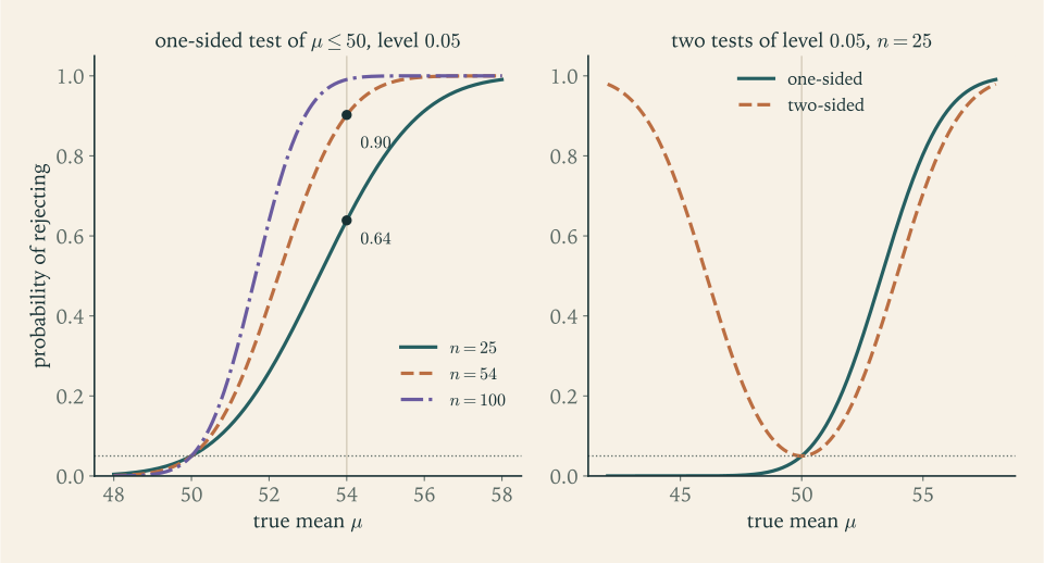
which is \(0.05\) at \(\mu=50\) , \(0.260\) at \(\mu=52\) , \(0.639\) at \(\mu=54\) , and \(0.912\) at \(\mu=56\) . An overfill of \(2\) grams would be detected only about a quarter of the time. If overfilling by \(4\) grams must be detected with probability \(0.90\) , the sample size has to satisfy \(1.645-4\sqrt n/10\le-z_{0.10}=-1.282\) , that is,

\[ n\ge\Bigl(\frac{(1.645+1.282)\times10}{4}\Bigr)^2\approx53.5, \]

so \(n=54\) packs. The left panel of Figure 8.1 shows the power curves for \(n=25\) , \(54\) , and \(100\) .

The general formula from this example is worth recording. Let \(\kappa\) be the type II error probability that can be tolerated at a shift \(\Delta\) , so that the required power there is \(1-\kappa\) . A one-sided level-\(\alpha\) test achieves it when

\[ n\ge\Bigl(\frac{(z_\alpha+z_\kappa)\,\sigma}{\Delta}\Bigr)^2 . \]

Halving the shift to be detected quadruples the sample size. A study planned without this calculation may have little chance of detecting the effect it is looking for.

8.2 The best test of one simple hypothesis against another

Example 8.1 assumed that rejecting for large \(\bar X\) was the right form of test. To prove such a claim, begin with the simplest problem, in which each hypothesis names a single distribution.

The lemma says that the evidence for \(H_1\) against \(H_0\) is ordered by the likelihood ratio \(f_1(x)/f_0(x)\) . The best test spends its allowance of type I error on the outcomes where that ratio is largest, where each unit of probability under \(H_0\) buys the most probability under \(H_1\) . Randomization, the constant \(\gamma\) on the boundary set, is needed only when the likelihood ratio takes a particular value with positive probability, as it does for discrete data; it lets the size be exactly \(\alpha\) and is of theoretical more than practical interest.

By the factorization theorem the likelihood ratio depends on the data only through a sufficient statistic, so the most powerful test does too (Exercise 19).

8.3 Composite alternatives and uniformly most powerful tests

The alternative \(p=0.8\) in Example 8.2 was arbitrary, and the form of the best test, reject for large \(X\) , did not depend on it: for any \(p_1>0.5\) the likelihood ratio is increasing in \(x\) . The same test is therefore most powerful against every alternative \(p_1>0.5\) simultaneously. The property behind this can be isolated.

A one-parameter exponential family \(h(x)\exp(\eta(\theta)T(x)-B(\theta))\) with \(\eta\) increasing has monotone likelihood ratio in \(T\) , since the ratio is \(\exp\bigl((\eta(\theta_2)-\eta(\theta_1))T(x)\bigr)\) times a constant. This covers the binomial, Poisson, and exponential families and the normal family with either parameter known. For a random sample the statistic is \(\sum T(x_i)\) .

The theorem justifies Example 8.1: the normal family with known variance has monotone likelihood ratio in \(\bar X\) , so the test rejecting for \(\bar X>53.29\) is UMP among all level-\(0.05\) tests of \(\mu\le50\) against \(\mu>50\) . No cleverer use of the 25 weights can do better against any \(\mu>50\) .

8.4 p-values

A test at a fixed level gives a binary report. It is more informative to say how extreme the data were.

A small p-value means that data as extreme as those observed would be unusual if \(H_0\) were true. The p-value is a statistic: a function of the data, with a sampling distribution. Its defining property is the following.

So the p-value is the smallest level at which the observed data would lead to rejection, and reporting it lets each reader apply a personal level. For the filling machine, \(z=1.75\) and the p-value is \(P(Z\ge1.75)\approx0.040\) : the test rejects at level \(0.05\) and would not reject at level \(0.01\) .

8.5 Tests and confidence sets are one construction

The interval \((9.866,10.334)\) of Example 7.1 contains \(10\) , and the test of \(\mu=10\) in Example 8.4 did not reject. This is not a coincidence.

A \(1-\alpha\) confidence set is the set of parameter values that a level-\(\alpha\) test would not reject. The two-sided \(t\) -test rejects \(\mu=\mu_0\) exactly when \(\lvert\bar x-\mu_0\rvert>t_{n-1,\alpha/2}\,s/\sqrt n\) , that is, exactly when \(\mu_0\) lies outside the \(t\) interval. The Clopper–Pearson interval of Theorem 7.4 is the inversion of a pair of one-sided binomial tests. Good tests give good confidence sets: inverting a UMP one-sided test gives a confidence bound that is least likely to include false values.

The correspondence also shows what each presentation adds. A test answers a question about one parameter value. The confidence set answers it for all values at once, and so displays the size of the effect and the precision with which it is known. For the two processes, “\(p=0.0009\) ” says the difference is not zero; the interval \((0.39,1.23)\) says how large it plausibly is.

8.6 Likelihood ratio tests

When both hypotheses are composite and no UMP test exists, a general recipe is to compare the best explanation of the data under \(H_0\) with the best explanation overall.

Since the numerator maximises over a subset, \(0\le\Lambda\le1\) . Values near one mean that restricting to \(H_0\) costs little likelihood; small values mean the unrestricted maximum is far better. For two simple hypotheses the rule reduces to the Neyman–Pearson test.

8.7 Many tests, and what significance does not mean

When several hypotheses are tested, the chance of at least one false rejection grows. With \(20\) independent tests of true null hypotheses, each at level \(0.05\) , the probability of at least one rejection is \(1-0.95^{20}\approx0.64\) . The Bonferroni argument of Proposition 7.5 applies directly: testing each of \(m\) hypotheses at level \(\alpha/m\) keeps the probability of any false rejection at most \(\alpha\) , whatever the dependence among the tests. For \(m=20\) and \(\alpha=0.05\) each test is run at level \(0.0025\) .

The same arithmetic governs any search through the data. Trying several test statistics, several subsets of the observations, or several definitions of the outcome, and reporting the one with the smallest p-value, is a multiple-testing procedure whose error rate is not the nominal one. The level of a test is guaranteed only when the hypothesis and the test were fixed before the data were examined.

Finally, statistical significance is a statement about sampling variability and nothing more. A rejected null hypothesis may correspond to a difference too small to matter, and a non-rejected one to a difference that matters but was measured too imprecisely to detect. The questions that matter in practice, how large is the effect and how well is it determined, are answered by the estimate and its confidence interval, with the power function describing what the study could and could not have seen.

So far every sampling distribution used in a test or an interval has been exact. The models where that is possible are few. The next chapter develops the approximations that extend these methods to all regular models.

Exercises

1. Define size, level, and power. For the test of Example 8.1 that rejects when \(\bar x>53.29\) , compute the probability of a type II error when \(\mu=52\) and when \(\mu=56\) .

   Answer

   Size is the largest rejection probability under \(H_0\) ; a test has level \(\alpha\) if its size is at most \(\alpha\) ; power is the rejection probability under an alternative. The type II error probability is \(1-\beta(\mu)\) : \(1-0.260=0.740\) at \(\mu=52\) and \(1-0.912=0.088\) at \(\mu=56\) .

2. For the two-sided level-\(\alpha\) \(z\) -test of \(H_0:\mu=\mu_0\) with known \(\sigma\) , show that the power is \(\Phi(-z_{\alpha/2}+\delta)+\Phi(-z_{\alpha/2}-\delta)\) with \(\delta=\sqrt n(\mu-\mu_0)/\sigma\) , and evaluate it for the filling machine at \(\mu=54\) .

   Answer

   \(Z=\sqrt n(\bar X-\mu_0)/\sigma\sim N(\delta,1)\) , so \(P(Z>z_{\alpha/2})=\Phi(-z_{\alpha/2}+\delta)\) and \(P(Z<-z_{\alpha/2})=\Phi(-z_{\alpha/2}-\delta)\) . For the filling machine at \(\mu=54\) , \(\delta=2\) and the power is \(\Phi(0.04)+\Phi(-3.96)\approx0.516\) .

3. Derive the sample-size formula \(n\ge\bigl((z_\alpha+z_\kappa)\sigma/\Delta\bigr)^2\) for a one-sided \(z\) -test with power \(1-\kappa\) at a shift \(\Delta\) , and compute \(n\) for \(\alpha=0.01\) , power \(0.95\) , \(\sigma=10\) , and \(\Delta=5\) .

   Solution

   The test rejects when \(Z=\sqrt n(\bar X-\mu_0)/\sigma>z_\alpha\) . Under a true mean \(\mu_0+\Delta\) with \(\Delta>0\) , \(Z\sim N(\sqrt n\Delta/\sigma,\ 1)\) , so the power is

   \[ P(Z>z_\alpha)=1-\Phi\Bigl(z_\alpha-\frac{\sqrt n\,\Delta}{\sigma}\Bigr). \]

   The requirement that this be at least \(1-\kappa\) is \(\Phi(z_\alpha-\sqrt n\Delta/\sigma)\le\kappa\) . Since \(\Phi(-z_\kappa)=\kappa\) and \(\Phi\) is increasing, this holds exactly when

   \[ z_\alpha-\frac{\sqrt n\,\Delta}{\sigma}\le-z_\kappa,\qquad\text{that is,}\qquad \sqrt n\ge\frac{(z_\alpha+z_\kappa)\sigma}{\Delta}, \]

   and squaring gives the formula.

   For \(\alpha=0.01\) and power \(0.95\) : \(z_{0.01}\approx2.326\) and \(z_{0.05}\approx1.645\) . With \(\sigma=10\) and \(\Delta=5\) ,

   \[ n\ge\Bigl(\frac{(2.326+1.645)\times10}{5}\Bigr)^2=(7.942)^2\approx63.1, \]

   so \(n=64\) . The sample size depends on the shift only through the standardised effect \(\Delta/\sigma=0.5\) , and both error rates enter through their normal quantiles: tightening either one increases the sum \(z_\alpha+z_\kappa\) and hence \(n\) .

4. A single observation \(X\) comes from \(N(0,1)\) under \(H_0\) and from \(N(1,1)\) under \(H_1\) . Find the most powerful test of level \(0.05\) and its power, and state the corresponding test based on a random sample of size \(n\) .

   Answer

   The likelihood ratio \(e^{x-1/2}\) is increasing in \(x\) , so the most powerful test rejects when \(X>1.645\) ; its power is \(1-\Phi(0.645)\approx0.260\) . For a sample of size \(n\) , reject when \(\sqrt n\,\bar X>1.645\) ; the power is \(1-\Phi(1.645-\sqrt n)\) .

5. A single observation \(X\) comes from \(N(0,1)\) under \(H_0\) and from \(N(0,4)\) under \(H_1\) . Show that the likelihood ratio is an increasing function of \(x^2\) , find the most powerful level-\(0.05\) test, and compute its power.

   Solution

   The densities are \(f_0(x)=(2\pi)^{-1/2}e^{-x^2/2}\) and \(f_1(x)=(8\pi)^{-1/2}e^{-x^2/8}\) . Their ratio is

   \[ \frac{f_1(x)}{f_0(x)}=\frac12\exp\Bigl(\frac{x^2}{2}-\frac{x^2}{8}\Bigr)=\frac12\exp\Bigl(\frac{3x^2}{8}\Bigr), \]

   a strictly increasing function of \(x^2\) . By the Neyman–Pearson lemma the most powerful test rejects when the ratio exceeds a constant, that is, when \(x^2>c^2\) , or \(\lvert x\rvert>c\) . The distribution is continuous, so no randomization is needed.

   Size: under \(H_0\) , \(P(\lvert X\rvert>c)=0.05\) gives \(c=z_{0.025}=1.960\) .

   Power: under \(H_1\) , \(X/2\) is standard normal, so

   \[ P_1(\lvert X\rvert>1.960)=P(\lvert Z\rvert>0.980)=2\bigl(1-\Phi(0.980)\bigr)\approx0.327 . \]

   Here the alternative differs from the null in spread, not in location, and the most powerful test is two-sided as a result: observations far from zero in either direction are relatively more probable under the wider distribution. The form of the best test is dictated by the likelihood ratio, not by a habit of rejecting for large values. The power is low because a single observation carries little information about a variance.

6. A single Poisson count \(X\) has mean \(1\) under \(H_0\) and mean \(3\) under \(H_1\) . Construct the most powerful test of size exactly \(0.05\) , including its randomization probability, and compute its power.

   Solution

   The likelihood ratio is

   \[ \frac{f_1(x)}{f_0(x)}=\frac{e^{-3}3^x/x!}{e^{-1}1^x/x!}=e^{-2}\,3^x, \]

   increasing in \(x\) , so the most powerful test rejects for large \(x\) and randomizes on a boundary value.

   Under \(H_0\) (mean \(1\) ): \(P_0(X\ge4)\approx0.0190\) and \(P_0(X\ge3)\approx0.0803\) , with \(P_0(X=3)\approx0.0613\) . Rejecting for \(X\ge4\) uses less than the allowance \(0.05\) and rejecting for \(X\ge3\) exceeds it, so reject when \(X\ge4\) and reject with probability \(\gamma\) when \(X=3\) , where

   \[ 0.0190+\gamma(0.0613)=0.05,\qquad\gamma=\frac{0.05-0.0190}{0.0613}\approx0.506 . \]

   Power, under \(H_1\) (mean \(3\) ): \(P_1(X\ge4)\approx0.3528\) and \(P_1(X=3)\approx0.2240\) , so

   \[ E_1\phi=0.3528+0.506\times0.2240\approx0.466 . \]

   By Theorem 8.2 no test of level \(0.05\) has higher power against a mean of \(3\) . The nonrandomized test “reject when \(X\ge4\) ” has size \(0.0190\) and power \(0.3528\) ; the randomized test gains about \(0.11\) in power by spending the remaining \(0.031\) of size on part of the outcome \(X=3\) .

7. Prove that if a most powerful level-\(\alpha\) test of \(f_0\) against \(f_1\) has power exactly \(\alpha\) with \(0<\alpha<1\) , then \(f_0=f_1\) except on a set of probability zero.

   Hint

   Compare with \(\phi'\equiv\alpha\) and examine when the integral in the proof of Theorem 8.2 can vanish: \(\int(\phi-\alpha)(f_1-kf_0)\,dx=0\) with a nonnegative integrand forces \(f_1=kf_0\) wherever \(\phi\ne\alpha\) , hence almost everywhere when \(0<\alpha<1\) ; integrate both sides to find \(k=1\) .

8. Show that the binomial family has monotone likelihood ratio in \(x\) and that the uniform family on \((0,\theta)\) has monotone likelihood ratio in the sample maximum, and state the form of the UMP test of \(H_0:p\le p_0\) against \(H_1:p>p_0\) .

   Hint

   For the binomial, \(f(x;p_2)/f(x;p_1)\) is a constant times \(\bigl(\frac{p_2(1-p_1)}{p_1(1-p_2)}\bigr)^x\) with base greater than one. For the uniform, the ratio is \((\theta_1/\theta_2)^n\) when the maximum is below \(\theta_1\) and infinite when it lies between \(\theta_1\) and \(\theta_2\) . The UMP test rejects for large \(X\) , with randomization at the boundary value.

9. Ten observations from \(N(0,\sigma^2)\) have \(\sum x_i^2=85\) . Give the UMP level-\(0.05\) test of \(H_0:\sigma^2\le4\) against \(H_1:\sigma^2>4\) , carry it out, and report the p-value.

   Answer

   The family has monotone likelihood ratio in \(\sum x_i^2\) , so reject when \(\sum x_i^2/4>\chi^2_{10,0.05}\approx18.31\) . The statistic is \(85/4=21.25\) : reject. The p-value is \(P(\chi^2_{10}\ge21.25)\approx0.019\) .

10. For the filling machine with \(n=25\) , compute the power of the one-sided level-\(0.05\) test and of the two-sided level-\(0.05\) test at \(\mu=46\) and at \(\mu=54\) , and explain what the four numbers show about the existence of a UMP test against \(\mu\ne50\) .

    Solution

    With \(n=25\) and \(\sigma=10\) , \(\delta=\sqrt{25}(\mu-50)/10=(\mu-50)/2\) , which is \(-2\) at \(\mu=46\) and \(+2\) at \(\mu=54\) .

    One-sided test (reject when \(Z>1.645\) ): the power is \(1-\Phi(1.645-\delta)\) . At \(\mu=54\) : \(1-\Phi(-0.355)\approx0.639\) . At \(\mu=46\) : \(1-\Phi(3.645)\approx0.0001\) .

    Two-sided test (reject when \(\lvert Z\rvert>1.960\) ): by Exercise 8.2 the power is \(\Phi(-1.960+\delta)+\Phi(-1.960-\delta)\) , which is symmetric in \(\delta\) . At \(\mu=54\) and at \(\mu=46\) : \(\Phi(0.04)+\Phi(-3.96)\approx0.516\) .

    At \(\mu=54\) the one-sided test is better, \(0.639\) against \(0.516\) , and by Theorem 8.5 nothing of level \(0.05\) beats \(0.639\) there. At \(\mu=46\) the mirror-image one-sided test, rejecting when \(Z<-1.645\) , also has power \(0.639\) , and nothing beats that either. A test that was UMP against \(\mu\ne50\) would need power \(0.639\) at both points. But the only tests reaching \(0.639\) at \(\mu=54\) are essentially the upper one-sided test, whose power at \(\mu=46\) is \(0.0001\) . So no UMP test exists for the two-sided problem. The two-sided test gives up about \(0.12\) of power on each side to obtain reasonable power on both.

11. In Example 8.1 the observed mean is \(53.5\) . Compute the one-sided and the two-sided p-values, and explain when the two-sided value is the appropriate one.

    Answer

    \(z=1.75\) . One-sided: \(P(Z\ge1.75)\approx0.040\) . Two-sided: \(P(\lvert Z\rvert\ge1.75)\approx0.080\) . The two-sided value is appropriate when departures in either direction would have been reported as evidence against \(H_0\) , and the direction was not fixed before seeing the data.

12. Explain what is wrong with each statement: (a) “The p-value is \(0.03\) , so there is a \(3\%\) chance that the null hypothesis is true.” (b) “The p-value is \(0.35\) , so the null hypothesis has been confirmed.” (c) “The p-value is \(0.0001\) , so the effect is large.”

    Solution

    (a) The p-value is computed under the assumption that \(H_0\) is true; it is the probability of data at least as extreme as those observed, given \(H_0\) . It is not a probability of \(H_0\) given the data. In the framework of this chapter \(H_0\) is a fixed statement that is true or false, and no probability is assigned to it. Converting \(P(\text{data}\mid H_0)\) into \(P(H_0\mid\text{data})\) requires Bayes’ rule and a prior probability for \(H_0\) .

    (b) A p-value of \(0.35\) says the data are unremarkable under \(H_0\) . They may be equally unremarkable under many alternatives. Failing to reject is evidence for \(H_0\) only to the extent that the test had high power against the alternatives of interest; otherwise it reflects the limits of the study. Theorem 8.7 also shows that under \(H_0\) the p-value is uniformly distributed, so a value near \(0.35\) is no more “confirming” than one near \(0.9\) or \(0.1\) .

    (c) The p-value depends on the estimated effect and on its standard error, which shrinks with sample size. A minute effect measured on a very large sample gives a tiny p-value. With \(n=10^6\) and \(\sigma=1\) , a mean shift of \(0.004\) gives \(z=4\) and a two-sided p-value below \(0.0001\) . The size of an effect is read from the estimate and its confidence interval.

13. A study of nine measurements with \(\sigma=0.3\) tests \(H_0:\mu=10\) with a two-sided level-\(0.05\) \(z\) -test and does not reject. Compute the power of this test when the true mean is \(10.1\) , and explain what the result implies about interpreting the non-rejection.

    Solution

    The standard error is \(0.3/\sqrt9=0.1\) , so a true mean of \(10.1\) gives \(\delta=(10.1-10)/0.1=1\) . By Exercise 8.2 the power of the two-sided level-\(0.05\) test is

    \[ \Phi(-1.960+1)+\Phi(-1.960-1)=\Phi(-0.960)+\Phi(-2.960)\approx0.1685+0.0015=0.170 . \]

    If the true mean were \(10.1\) , a full standard error away from the hypothesised value, the test would reject only \(17\%\) of the time and fail to reject \(83\%\) of the time. Non-rejection is therefore the expected outcome whether the mean is \(10\) or \(10.1\) , and it cannot discriminate between them. The correct summary is not “the mean is \(10\) ” but “the data are compatible with a range of means”, and the confidence interval states the range: with \(\bar x=10.1\) it is \(10.1\pm0.196\) , which includes both \(10\) and \(10.2\) . To have power \(0.9\) against a shift of \(0.1\) would need \(n\ge\bigl((1.960+1.282)\times0.3/0.1\bigr)^2\approx95\) measurements.

14. For \(X\sim\operatorname{Binomial}(10,p)\) and the test of \(H_0:p=0.5\) against \(H_1:p>0.5\) based on large \(X\) , list the attainable p-values for \(x=6,\dots,10\) , and verify directly that \(P_{0.5}(p(X)\le0.05)\le0.05\) .

    Solution

    The p-value for an observed \(x\) is \(p(x)=P_{0.5}(X\ge x)\) , computed from the \(\operatorname{Binomial}(10,0.5)\) distribution:

    \[ p(6)=\tfrac{386}{1024}\approx0.377,\quad p(7)=\tfrac{176}{1024}\approx0.172,\quad p(8)=\tfrac{56}{1024}\approx0.0547,\quad p(9)=\tfrac{11}{1024}\approx0.0107,\quad p(10)=\tfrac{1}{1024}\approx0.0010 . \]

    The p-value is a decreasing function of \(x\) , and it is at most \(0.05\) exactly when \(x\ge9\) . Therefore

    \[ P_{0.5}\bigl(p(X)\le0.05\bigr)=P_{0.5}(X\ge9)=\tfrac{11}{1024}\approx0.0107\le0.05 , \]

    as Theorem 8.7 guarantees. The inequality is far from an equality: because the p-value jumps from \(0.0547\) to \(0.0107\) with nothing in between, a test at level \(0.05\) actually has size \(0.0107\) . With discrete data the p-value is conservative: its distribution under \(H_0\) is not uniform but is stochastically larger than uniform. The general statement \(P(p\le u)\le u\) becomes an equality only at the attainable values of \(u\) , for example \(P_{0.5}(p(X)\le0.0547)=0.0547\) .

15. Invert the UMP test of Example 8.3, for a general boundary value \(\theta_0\) in place of \(3\) , to obtain a \(95\%\) lower confidence bound for the mean lifetime, and check that it agrees with Exercise 7.5.

    Hint

    The test of \(\theta\le\theta_0\) does not reject when \(2\sum x_i/\theta_0\le31.41\) , that is, when \(\theta_0\ge2\sum x_i/31.41\) . By Theorem 8.8 the set of such \(\theta_0\) is a \(95\%\) confidence set: \([2\sum x_i/31.41,\infty)=[2.67,\infty)\) .

16. For a random sample from \(\operatorname{Exp}(\lambda)\) , derive the likelihood ratio statistic for \(H_0:\lambda=\lambda_0\) against \(H_1:\lambda\ne\lambda_0\) as a function of \(\lambda_0\bar x\) , describe the shape of the rejection region, and evaluate \(-2\log\Lambda\) for \(n=10\) , \(\bar x=4.2\) , \(\lambda_0=1/3\) .

    Solution

    The likelihood is \(L(\lambda)=\lambda^n e^{-\lambda n\bar x}\) , maximised over \(\lambda>0\) at \(\hat\lambda=1/\bar x\) with \(L(\hat\lambda)=\bar x^{-n}e^{-n}\) . The null hypothesis is simple, so the numerator is \(L(\lambda_0)\) , and

    \[ \Lambda=\frac{\lambda_0^n e^{-\lambda_0n\bar x}}{\bar x^{-n}e^{-n}}=\bigl(u\,e^{1-u}\bigr)^n,\qquad u=\lambda_0\bar x . \]

    The function \(u\mapsto ue^{1-u}\) increases on \((0,1)\) , equals \(1\) at \(u=1\) , and decreases on \((1,\infty)\) . So \(\Lambda\le c\) exactly when \(u\le a\) or \(u\ge b\) , for two numbers \(a<1<b\) with \(ae^{1-a}=be^{1-b}\) . The test rejects when \(\lambda_0\bar x\) is too small or too large, that is, when the sample mean is far from the hypothesised mean \(1/\lambda_0\) in either direction.

    The region is not symmetric about \(u=1\) and it does not place equal probability in the two tails: since \(ue^{1-u}\) falls more steeply to the left of \(1\) than to the right, \(b-1>1-a\) . Under \(H_0\) , \(2n\lambda_0\bar X\sim\chi^2_{2n}\) , so exact critical values can be found from the chi-square distribution.

    For the data, \(u=4.2/3=1.4\) and

    \[ -2\log\Lambda=-2n\bigl(\log u+1-u\bigr)=-20(\log1.4-0.4)\approx-20(0.3365-0.4)=1.27 . \]

    Chapter 9 shows that this statistic is approximately \(\chi^2_1\) under \(H_0\) ; the value \(1.27\) is well below the \(5\%\) point \(3.84\) , so \(\lambda_0=1/3\) is not rejected.

17. For two independent normal samples with a common unknown variance, show that the likelihood ratio statistic for \(H_0:\mu_1=\mu_2\) satisfies \(\Lambda^{2/N}=1/\bigl(1+t^2/(N-2)\bigr)\) , where \(N=m+n\) and \(t\) is the pooled two-sample statistic.

    Hint

    Proceed as in Example 8.5. The unrestricted variance estimate is \(\frac1N(SS_X+SS_Y)\) and the restricted one adds the between-sample term \(\frac{mn}{N}(\bar x-\bar y)^2\) to the numerator; then use \(t^2=\frac{mn}{N}(\bar x-\bar y)^2\big/\bigl((SS_X+SS_Y)/(N-2)\bigr)\) .

18. Twenty hypotheses are tested and the three smallest p-values are \(0.001\) , \(0.02\) , and \(0.04\) . Which are rejected by the Bonferroni procedure at overall level \(0.05\) ? What is the probability of at least one false rejection if all twenty null hypotheses are true and each is tested at level \(0.05\) independently?

    Answer

    The Bonferroni threshold is \(0.05/20=0.0025\) ; only the hypothesis with \(p=0.001\) is rejected. With twenty independent tests of true hypotheses at level \(0.05\) , the probability of at least one false rejection is \(1-0.95^{20}\approx0.64\) .

19. Let \(T\) be a sufficient statistic for a model containing \(\theta_0\) and \(\theta_1\) . Use the factorization theorem to show that the Neyman–Pearson test of \(\theta_0\) against \(\theta_1\) depends on the data only through \(T\) .

    Solution

    By the factorization theorem (Theorem 3.2) there are functions \(g\) and \(h\) with \(f(x;\theta)=g(T(x),\theta)h(x)\) for every \(\theta\) in the model, in particular for \(\theta_0\) and \(\theta_1\) . At any \(x\) with \(h(x)>0\) ,

    \[ \frac{f(x;\theta_1)}{f(x;\theta_0)}=\frac{g(T(x),\theta_1)\,h(x)}{g(T(x),\theta_0)\,h(x)}=\frac{g(T(x),\theta_1)}{g(T(x),\theta_0)}, \]

    a function of \(T(x)\) alone. Points with \(h(x)=0\) have density zero under both hypotheses and can be ignored.

    The Neyman–Pearson test of Theorem 8.2 is defined by comparing \(f(x;\theta_1)\) with \(kf(x;\theta_0)\) . The three cases \(f_1>kf_0\) , \(f_1=kf_0\) , \(f_1<kf_0\) are equivalent to \(g(T(x),\theta_1)\) being greater than, equal to, or less than \(k\,g(T(x),\theta_0)\) , which depends on \(x\) only through \(T(x)\) . So \(\phi(x)=\psi(T(x))\) for some function \(\psi\) .

    This is the testing counterpart of the Rao–Blackwell theorem: nothing is gained in power by looking at the data beyond a sufficient statistic. It also explains the form of the tests in this chapter, each of which is based on the sufficient statistic of its model: \(\bar X\) for the normal mean, the count for the binomial, the total for the exponential.