The nine length measurements of Chapter 5 have mean \(10.1\) millimetres. Reported alone, that number invites two opposite misreadings: that the true length is \(10.1\) , or that nothing can be said because the measurements scatter. Both are wrong, and what lies between them is a statement of the form “the true length is between \(9.87\) and \(10.33\) ”, together with a precise account of how much trust that statement deserves.
The account cannot be “the probability that the length lies in this range is \(0.95\) ”, at least not within the framework used so far, because the length is a fixed unknown constant and the two endpoints, once computed, are fixed known constants. Nothing in the sentence is random. What is random is the procedure: before the data are collected, the endpoints are random variables, and one can ask how often the random range they define will contain the fixed truth. A confidence interval is a procedure for which that frequency is high, whatever the truth is.
This chapter defines the idea, builds confidence sets from the pivots of Chapter 2, and examines what to do when no exact pivot exists. It also separates three statements that are easily confused: where the parameter is, where the data are, and where the next observation will be.
7.1 What a confidence set claims
Definition 7.1 (confidence set). Let \(C(X)\) be a subset of the parameter space determined by the data. \(C(X)\) is a confidence set for \(\theta\) with confidence level \(1-\alpha\) if
The function \(\theta\mapsto P_\theta(\theta\in C(X))\) is the coverage probability, and its infimum over \(\Theta\) is the confidence coefficient. When \(C(X)\) is an interval \([L(X),U(X)]\) it is a confidence interval; a set of the form \((-\infty,U(X)]\) or \([L(X),\infty)\) gives an upper or lower confidence bound.
In the probability \(P_\theta(\theta\in C(X))\) the random object is the set \(C(X)\) . The parameter \(\theta\) appears twice, as the fixed point being covered and as the index of the law under which the data are generated, and the inequality must hold for every value it could have. That requirement is what makes the statement useful: since the guarantee holds whichever \(\theta\) is true, it holds for the true one without our knowing which that is.
Figure 7.1 shows the idea in a simulation. On the left is the sampling distribution of the mean of nine measurements from \(N(10,0.3^2)\) : the mean falls within \(0.196\) of the truth with probability \(0.95\) . On the right, the experiment was run \(50\) times, and each time a \(95\%\) interval was computed by the method of Example 7.1 below. The intervals differ in location and in length from run to run. Most of them contain the true mean \(10\) ; in this simulation \(5\) of the \(50\) do not.
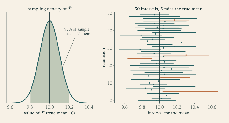
Five misses in fifty is \(10\%\) , not \(5\%\) , and that is not an error. The number of misses in \(50\) independent runs is binomial with mean \(2.5\) , and a count of five or more has probability about \(0.10\) . The confidence level is a property of the procedure over indefinitely many repetitions. It does not promise that exactly \(95\%\) of any finite batch will cover, and it says nothing at all about which particular intervals are the failures. An analyst holding one of the five failing intervals has no way to know it.
Common mistake. Saying, after computing the interval \((9.87,10.33)\) , that “\(\mu\) lies in it with probability \(0.95\) ”. Before the data, \(P_\mu(L(X)\le\mu\le U(X))=0.95\) is a statement about random endpoints. After the data, the event \(9.87\le\mu\le10.33\) is either true or false, and no probability in the model attaches to it. The number \(0.95\) describes the reliability of the method that produced the interval. A probability statement about \(\mu\) itself requires treating \(\mu\) as random, which is the Bayesian approach of Chapter 11.
7.2 Inverting a pivot
A pivot \(Q(X,\theta)\) has a known distribution, so one can choose a set \(A\) that it falls in with probability \(1-\alpha\) . The values of \(\theta\) that put the observed pivot inside \(A\) form a confidence set.
Theorem 7.2 (pivot inversion). Let \(Q(X,\theta)\) be a pivot and let \(A\) be a set with \(P(Q(X,\theta)\in A)\ge1-\alpha\) . Define
Then \(C(X)\) is a confidence set with level \(1-\alpha\) , and its coverage probability is the same for every \(\theta\) .
Proof. By the definition of \(C\) , the event \(\theta\in C(X)\) is the same event as \(Q(X,\theta)\in A\) . Under \(P_\theta\) the latter has a probability that does not depend on \(\theta\) , because \(Q\) is a pivot, and that probability is at least \(1-\alpha\) by the choice of \(A\) .
The theorem is one line long because all the work is in finding the pivot. When \(Q(x,\theta)\) is monotone in a real parameter \(\theta\) and \(A=[a,b]\) is an interval, the set \(C(x)\) is an interval whose endpoints are found by solving \(Q(x,\theta)=a\) and \(Q(x,\theta)=b\) .
Example 7.1: Intervals for a normal mean
Let \(X_1,\dots,X_n\) be a random sample from \(N(\mu,\sigma^2)\) .
Known \(\sigma\) . The pivot \(\sqrt n(\bar X-\mu)/\sigma\) is standard normal, so it lies between \(-z_{\alpha/2}\) and \(z_{\alpha/2}\) with probability \(1-\alpha\) . Solving the two inequalities for \(\mu\) ,
If the lengths are known to have \(\sigma=0.3\) , then with \(n=9\) , \(\bar x=10.1\) , and \(z_{0.025}=1.960\) , the \(95\%\) interval is \(10.1\pm1.960(0.1)\) , that is, \((9.904,\ 10.296)\) .
Unknown \(\sigma\) . The pivot is now \(\sqrt n(\bar X-\mu)/S\sim t_{n-1}\) (Corollary 2.6), and the same algebra gives
For the lengths, \(s^2=0.0925\) , so \(s\approx0.3041\) and \(s/\sqrt9\approx0.1014\) ; with \(t_{8,0.025}\approx2.306\) the half-width is \(2.306\times0.1014\approx0.234\) and the \(95\%\) interval is \((9.866,\ 10.334)\) .
The second interval is wider, although the estimate of \(\sigma\) is close to \(0.3\) . The extra width comes from the quantile, \(2.306\) instead of \(1.960\) , and reflects that \(S\) could easily have come out too small. With unknown \(\sigma\) the length of the interval is itself random, as the right panel of Figure 7.1 shows.
A one-sided version uses one tail: \(P(\sqrt n(\bar X-\mu)/S\le t_{n-1,\alpha})=1-\alpha\) gives the lower confidence bound \(\mu\ge\bar X-t_{n-1,\alpha}S/\sqrt n\) . For the lengths, \(t_{8,0.05}\approx1.860\) and the \(95\%\) lower bound is \(10.1-1.860(0.1014)\approx9.911\) .
Example 7.2: An interval for a variance
For the same normal sample, \((n-1)S^2/\sigma^2\sim\chi^2_{n-1}\) is a pivot involving only \(\sigma^2\) . With probability \(1-\alpha\) ,
and since the pivot is decreasing in \(\sigma^2\) , inverting reverses the order of the endpoints:
For the lengths, \((n-1)s^2=0.74\) , and the \(\chi^2_8\) quantiles are \(\chi^2_{8,0.025}\approx17.535\) and \(\chi^2_{8,0.975}\approx2.180\) . The \(95\%\) interval for \(\sigma^2\) is
and taking square roots, the interval for \(\sigma\) is \((0.205,\ 0.583)\) . The upper limit for \(\sigma\) is nearly three times the lower. Nine observations estimate a mean tolerably and a standard deviation poorly. The interval is far from symmetric about \(s=0.304\) , because the chi-square distribution is skewed.
Taking square roots was legitimate because a confidence set transforms with the parameter: if \(\theta\in C(X)\) with probability at least \(1-\alpha\) , then \(g(\theta)\in g(C(X))\) with at least that probability, for any function \(g\) . For an increasing \(g\) and an interval, the image is the interval between the images of the endpoints.
Example 7.3: Exponential lifetimes and a uniform endpoint
Exponential rate. Ten components have lifetimes that are a random sample from \(\operatorname{Exp}(\lambda)\) , with total \(\sum x_i=42.0\) hours. By Example 2.4, \(2\lambda\sum X_i\sim\chi^2_{20}\) , whose lower and upper \(2.5\%\) points are \(9.591\) and \(34.170\) . Solving \(9.591\le2\lambda(42.0)\le34.170\) for \(\lambda\) gives the \(95\%\) interval
and, taking reciprocals, the interval \((2.46,\ 8.76)\) hours for the mean lifetime \(1/\lambda\) , around the point estimate \(\bar x=4.2\) .
Uniform endpoint. For a random sample of size \(n\) from the uniform distribution on \((0,\theta)\) , \(M/\theta\) has distribution function \(u^n\) on \((0,1)\) (Example 2.3). For any \(0<a<b\le1\) with \(b^n-a^n=1-\alpha\) , the event \(a\le M/\theta\le b\) has probability \(1-\alpha\) , and inverting gives the interval \([M/b,\ M/a]\) for \(\theta\) . There are infinitely many such pairs. Taking \(b=1\) and \(a=\alpha^{1/n}\) gives
and for the five observations with \(M=3.0\) and \(\alpha=0.05\) this is \([3.0,\ 3.0/0.549]=[3.0,\ 5.46]\) . The equal-tailed choice \(a=0.025^{1/5}\) , \(b=0.975^{1/5}\) gives \([3.02,\ 6.27]\) , which is longer by about a third. Exercise 6 shows that \(b=1\) always gives the shortest interval of this family. The equal-tailed interval also has the odd feature of excluding values just above the largest observation, which are the best-supported values of all.
7.3 Which interval? Length, tails, and shape
A pivot determines a family of confidence sets, one for each choice of the set \(A\) . The uniform example shows that the choice matters. A natural criterion is expected length: among procedures with the same coverage, a shorter interval is more informative.
Proposition 7.3 (symmetric pivots). Let \(Q\) have a density \(g\) on \(\mathbb R\) that is symmetric about zero, positive everywhere, and nonincreasing on \([0,\infty)\) , and let \(c\) satisfy \(P(-c\le Q\le c)=1-\alpha\) . Then every interval \([a,b]\) with \(P(a\le Q\le b)\ge1-\alpha\) has length at least \(2c\) .
Proof. Let \([a,b]\) have midpoint \(m\) and half-length \(h\) ; by symmetry of \(g\) it suffices to treat \(m\ge0\) . Define \(G(m)=\int_{m-h}^{m+h}g(q)\,dq\) . Then \(G'(m)=g(m+h)-g(m-h)\) . Since \(m\ge0\) and \(h>0\) , we have \(\lvert m+h\rvert\ge\lvert m-h\rvert\) , and because \(g\) is symmetric and nonincreasing in \(\lvert q\rvert\) , \(g(m+h)\le g(m-h)\) . So \(G\) is nonincreasing on \([0,\infty)\) and \(P(a\le Q\le b)=G(m)\le G(0)=P(-h\le Q\le h)\) . If \(h<c\) then \(P(-h\le Q\le h)<P(-c\le Q\le c)=1-\alpha\) because \(g\) is positive on \((h,c)\) . Hence an interval with probability at least \(1-\alpha\) must have \(h\ge c\) .
For the normal and \(t\) pivots the interval for \(\mu\) has length \((b-a)\sigma/\sqrt n\) or \((b-a)S/\sqrt n\) , so the equal-tailed intervals of Example 7.1 are the shortest that those pivots can produce. For a skewed pivot the equal-tailed choice is a convention, not an optimum. In Example 7.2 a shorter interval for \(\sigma^2\) exists, about \(18\%\) shorter, obtained by putting almost all of \(\alpha\) in the lower tail of the chi-square distribution; the equal-tailed interval is used because the tail areas are easy to state and each tail error has the same probability.
Three things control the length of an interval, and all are visible in the half-width \(z_{\alpha/2}\sigma/\sqrt n\) . Higher confidence costs length through the quantile: moving from \(95\%\) to \(99\%\) replaces \(1.960\) by \(2.576\) . More variable data cost length through \(\sigma\) . More data buy length through \(\sqrt n\) : to halve an interval, quadruple the sample. Solving the half-width for \(n\) gives the sample size needed for a target precision \(d\) , namely \(n\ge(z_{\alpha/2}\sigma/d)^2\) .
7.4 Discrete data: guaranteed coverage without a pivot
For a binomial count the method breaks down. The count takes only finitely many values, with probabilities that change with \(p\) , and there is no pivot with a continuous, parameter-free distribution to invert. An interval computed from the count alone cannot have coverage exactly \(1-\alpha\) at every \(p\) : as \(p\to0\) the count is \(0\) with probability tending to one, so the coverage tends to \(1\) or to \(0\) according to whether the interval assigned to a count of zero reaches down to \(p\) or not. The definition of a confidence set can still be met, with inequality in place of equality.
Let \(X\sim\operatorname{Binomial}(n,p)\) . For each \(x\ge1\) the upper tail probability \(P_p(X\ge x)\) is continuous and strictly increasing in \(p\) , from \(0\) at \(p=0\) to \(1\) at \(p=1\) ; for each \(x\le n-1\) the lower tail \(P_p(X\le x)\) is strictly decreasing. Define the Clopper–Pearson limits by
with \(p_L(0)=0\) and \(p_U(n)=1\) . In words, \(p_L(x)\) is the smallest success probability under which a count as large as \(x\) is not too surprising, and \(p_U(x)\) is the largest under which a count as small as \(x\) is not too surprising.
Theorem 7.4 (Clopper–Pearson interval). For every \(p\in(0,1)\) ,
Proof. Fix \(p\) and consider the event \(p_L(X)>p\) . For \(x\ge1\) , because \(P_q(X\ge x)\) is increasing in \(q\) and equals \(\alpha/2\) at \(q=p_L(x)\) , the inequality \(p_L(x)>p\) holds exactly when \(P_p(X\ge x)<\alpha/2\) ; and \(p_L(0)=0\) is never greater than \(p\) . The function \(x\mapsto P_p(X\ge x)\) is nonincreasing, so the set of \(x\) with \(P_p(X\ge x)<\alpha/2\) is of the form \(\{x^\ast,x^\ast+1,\dots,n\}\) , where \(x^\ast\) is the smallest such \(x\) , or is empty. Therefore
The symmetric argument gives \(P_p(p_U(X)<p)<\alpha/2\) . The interval fails to cover \(p\) only if one of these two events occurs, so the probability of failure is less than \(\alpha\) .
The limits can be computed from beta quantiles: \(p_L(x)\) is the \(\alpha/2\) quantile of the \(\operatorname{Beta}(x,\,n-x+1)\) distribution and \(p_U(x)\) is the \(1-\alpha/2\) quantile of \(\operatorname{Beta}(x+1,\,n-x)\) . The interval is called exact, meaning that its guarantee is exact, not that its coverage equals \(1-\alpha\) . The coverage is strictly greater than \(1-\alpha\) for every \(p\) and varies with \(p\) : the price of a guarantee with discrete data is conservatism.
Example 7.4: Three defectives in twenty
For the inspector of Chapter 1, \(n=20\) and \(x=3\) . The \(95\%\) Clopper–Pearson limits are the \(0.025\) quantile of \(\operatorname{Beta}(3,18)\) and the \(0.975\) quantile of \(\operatorname{Beta}(4,17)\) :
A widely used shortcut treats \((\hat p-p)/\sqrt{\hat p(1-\hat p)/n}\) as approximately standard normal and reports \(\hat p\pm1.96\sqrt{\hat p(1-\hat p)/n}\) , the Wald interval. Here \(\hat p=0.15\) and the estimated standard error is \(\sqrt{0.15\times0.85/20}\approx0.0798\) , giving
The lower endpoint is negative, which no proportion can be. More seriously, the Wald interval does not have the coverage it claims. Its true coverage can be computed exactly by adding the binomial probabilities of those \(x\) whose interval contains \(p\) :
| True \(p\) | Wald coverage | Clopper–Pearson coverage |
|---|---|---|
| \(0.05\) | \(0.639\) | \(0.984\) |
| \(0.10\) | \(0.876\) | \(0.989\) |
| \(0.15\) | \(0.819\) | \(0.978\) |
| \(0.30\) | \(0.947\) | \(0.975\) |
| \(0.50\) | \(0.959\) | \(0.959\) |
For small \(p\) and \(n=20\) the nominal \(95\%\) Wald interval covers the truth far less often than advertised; at \(p=0.05\) it fails more than a third of the time, largely because the observation \(X=0\) , which has probability \(0.358\) , produces the degenerate interval \([0,0]\) . The Clopper–Pearson interval never falls below \(95\%\) and is often well above it. Chapter 9 derives a third interval, by inverting a different approximate pivot, that behaves better than the Wald interval without the full conservatism of the exact one.
7.5 Two samples, and several statements at once
Comparisons are the commonest use of intervals. Let \(X_1,\dots,X_m\) and \(Y_1,\dots,Y_n\) be independent random samples from \(N(\mu_1,\sigma^2)\) and \(N(\mu_2,\sigma^2)\) . By Exercise 2.6,
a pivot for the difference \(\mu_1-\mu_2\) , and inversion gives the pooled two-sample interval \(\bar X-\bar Y\pm t_{m+n-2,\alpha/2}\,S_p\sqrt{1/m+1/n}\) .
Example 7.5: Comparing two processes
Process A yields the eight strengths \(12.1\) , \(11.4\) , \(12.8\) , \(11.9\) , \(12.5\) , \(11.7\) , \(12.2\) , \(12.6\) , and process B the ten strengths \(11.2\) , \(11.9\) , \(10.8\) , \(11.5\) , \(11.0\) , \(11.8\) , \(11.3\) , \(10.9\) , \(11.6\) , \(11.4\) . The means are \(\bar x=12.15\) and \(\bar y=11.34\) , and the sums of squared deviations are \(1.580\) and \(1.244\) . Then
With \(t_{16,0.025}\approx2.120\) , the \(95\%\) interval for \(\mu_1-\mu_2\) is
The interval lies entirely above zero: at this confidence level the data are not compatible with equal means, and they indicate that process A is stronger by somewhere between \(0.4\) and \(1.2\) units. The calculation assumed equal variances. The two sample variances, \(0.226\) and \(0.138\) , differ by a factor of \(1.6\) , which with samples this small is unremarkable (Exercise 12). When the variances are clearly unequal the pooled pivot is no longer exact, and an approximate \(t\) pivot with estimated degrees of freedom, due to Welch, is used instead.
When several intervals are reported together, the chance that all of them cover is lower than the chance that each does.
Proposition 7.5 (Bonferroni). Let \(C_1(X),\dots,C_k(X)\) be confidence sets for \(\theta_1,\dots,\theta_k\) with levels \(1-\alpha_1,\dots,1-\alpha_k\) . Then
Proof. The complement of the event “all cover” is the union of the events \(\{\theta_j\notin C_j(X)\}\) , each of probability at most \(\alpha_j\) . The probability of a union is at most the sum of the probabilities.
No independence is required. To make \(k\) statements with joint confidence \(1-\alpha\) , construct each at level \(1-\alpha/k\) . For the nine lengths, joint \(95\%\) confidence for \(\mu\) and \(\sigma^2\) together is obtained from two \(97.5\%\) intervals (Exercise 14), each wider than its \(95\%\) counterpart. The proposition is also a warning about selective reporting: if twenty \(95\%\) intervals are computed and only the most striking is shown, the reader has no \(95\%\) guarantee for the one that is shown.
7.6 Where the next observation will fall
A confidence interval for \(\mu\) says where the mean of the population is. It does not say where an individual measurement will be. For that a different interval is needed.
Proposition 7.6 (prediction interval for a normal observation). Let \(X_1,\dots,X_n,X_{n+1}\) be a random sample from \(N(\mu,\sigma^2)\) , with \(\bar X\) and \(S\) computed from the first \(n\) . Then
and consequently \(P\bigl(\bar X-t_{n-1,\alpha/2}S\sqrt{1+1/n}\le X_{n+1}\le\bar X+t_{n-1,\alpha/2}S\sqrt{1+1/n}\bigr)=1-\alpha\) .
Proof. \(X_{n+1}\) is independent of \((\bar X,S)\) , and \(\bar X\) is independent of \(S\) by Theorem 2.5. So \(X_{n+1}-\bar X\) is normal with mean \(0\) and variance \(\sigma^2+\sigma^2/n\) , independent of \(S\) . Dividing by \(\sigma\sqrt{1+1/n}\) gives a standard normal variable, and \((n-1)S^2/\sigma^2\sim\chi^2_{n-1}\) independently; the ratio in the statement is a standard normal divided by the square root of an independent chi-square over its degrees of freedom.
The random quantity here is a pivot in an extended sense: it involves a future observation in place of a parameter, and both it and the interval endpoints are random. For the lengths, the \(95\%\) prediction interval is
more than three times as wide as the confidence interval \((9.866,10.334)\) for \(\mu\) . The two intervals answer different questions and behave differently as data accumulate. The half-width of the confidence interval is proportional to \(1/\sqrt n\) and shrinks to nothing. The half-width of the prediction interval tends to \(z_{\alpha/2}\sigma\) and no further: even with \(\mu\) and \(\sigma\) known exactly, a new measurement is uncertain by its own variability.
Common mistake. Reading a confidence interval for \(\mu\) as a range for individual values. About \(95\%\) of repeated intervals contain \(\mu\) ; nothing like \(95\%\) of observations fall in the confidence interval. Of the nine lengths themselves, only four lie in \((9.866,10.334)\) .
The construction of this chapter, a set of parameter values not contradicted by the data, has a twin. For each candidate value one can ask whether the data contradict it; the candidates that survive are the confidence set. That question, asked about one candidate at a time, is a hypothesis test, the subject of the next chapter.
Exercises
-
In the statement \(P_\theta(\theta\in C(X))\ge0.95\) , say which symbols denote random objects and which denote fixed ones, and explain why the inequality is required for every \(\theta\) and not only for the true one.
Hint
The set \(C(X)\) is random because the data are. The \(\theta\) inside the event is a fixed number, and the subscript on \(P_\theta\) says which law generates the data. Since the true \(\theta\) is unknown, a guarantee that held only for some values would be of no use: one could never tell whether it applied.
-
A random sample of size \(25\) from a normal population with known \(\sigma=10\) has mean \(54\) . Compute the \(95\%\) and \(99\%\) confidence intervals for \(\mu\) , and the sample size needed for a \(95\%\) interval of half-width at most \(1\) .
Answer
Standard error \(10/\sqrt{25}=2\) . \(95\%\) : \(54\pm1.960(2)=(50.08,\ 57.92)\) . \(99\%\) : \(54\pm2.576(2)=(48.85,\ 59.15)\) . Half-width \(1\) requires \(n\ge(1.960\times10)^2\approx384.2\) , so \(n=385\) .
-
Five observations from a normal population are \(4.1\) , \(5.2\) , \(3.8\) , \(4.9\) , \(4.5\) . Compute the sample mean and standard deviation and the \(95\%\) confidence interval for \(\mu\) .
Answer
\(\bar x=4.5\) , \(\sum(x_i-\bar x)^2=1.30\) , \(s^2=0.325\) , \(s\approx0.570\) . With \(t_{4,0.025}\approx2.776\) the half-width is \(2.776\times0.570/\sqrt5\approx0.708\) and the interval is \((3.79,\ 5.21)\) .
-
Derive the equal-tailed \(1-\alpha\) confidence interval for the standard deviation \(\sigma\) of a normal population from the chi-square pivot, justify the step from \(\sigma^2\) to \(\sigma\) , and evaluate the \(95\%\) interval for the data of Exercise 3.
Solution
By Theorem 2.5, \((n-1)S^2/\sigma^2\sim\chi^2_{n-1}\) for every \((\mu,\sigma^2)\) , so with probability exactly \(1-\alpha\)
\[ \chi^2_{n-1,1-\alpha/2}\le\frac{(n-1)S^2}{\sigma^2}\le\chi^2_{n-1,\alpha/2}. \]All quantities are positive, so taking reciprocals reverses the inequalities and multiplying by \((n-1)S^2\) preserves them:
\[ \frac{(n-1)S^2}{\chi^2_{n-1,\alpha/2}}\le\sigma^2\le\frac{(n-1)S^2}{\chi^2_{n-1,1-\alpha/2}}. \]The square root is strictly increasing on \((0,\infty)\) , so the event that \(\sigma^2\) lies between two positive numbers is the same event as \(\sigma\) lying between their square roots. The probability is unchanged, and
\[ \sqrt{\frac{(n-1)S^2}{\chi^2_{n-1,\alpha/2}}}\le\sigma\le\sqrt{\frac{(n-1)S^2}{\chi^2_{n-1,1-\alpha/2}}} \]is a \(1-\alpha\) confidence interval for \(\sigma\) .
For the data of Exercise 7.3, \((n-1)s^2=1.30\) , and the \(\chi^2_4\) quantiles are \(\chi^2_{4,0.025}\approx11.143\) and \(\chi^2_{4,0.975}\approx0.484\) . The interval for \(\sigma^2\) is \((1.30/11.143,\ 1.30/0.484)\approx(0.117,\ 2.684)\) and for \(\sigma\) it is \((0.342,\ 1.638)\) . The upper limit is almost five times the lower: five observations say very little about a standard deviation.
-
For the ten lifetimes of Example 7.3 with total \(42.0\) hours, compute a \(95\%\) lower confidence bound for the mean lifetime, and explain why a one-sided bound is the natural report when the concern is whether lifetimes are long enough.
Answer
A lower bound for the mean \(1/\lambda\) comes from an upper bound for \(\lambda\) : \(2\lambda(42.0)\le\chi^2_{20,0.05}\approx31.410\) with probability \(0.95\) , so \(1/\lambda\ge84/31.410\approx2.67\) hours. When only short lifetimes are a concern, an upper limit carries no useful guarantee and spending error probability on it weakens the lower one.
-
In the uniform model of Example 7.3, consider all intervals \([M/b,M/a]\) with \(0<a<b\le1\) and \(b^n-a^n=1-\alpha\) . Prove that the length is smallest when \(b=1\) .
Solution
The length of \([M/b,M/a]\) is \(M\,(1/a-1/b)\) , so it suffices to minimise \(\Lambda=1/a-1/b\) subject to \(b^n-a^n=1-\alpha\) and \(0<a<b\le1\) . The constraint determines \(a\) as a function of \(b\) : \(a(b)=\bigl(b^n-(1-\alpha)\bigr)^{1/n}\) , defined for \((1-\alpha)^{1/n}<b\le1\) . Differentiating the constraint, \(nb^{n-1}-na^{n-1}a'(b)=0\) , so
\[ a'(b)=\frac{b^{n-1}}{a^{n-1}}. \]Then
\[ \frac{d\Lambda}{db}=-\frac{a'(b)}{a^2}+\frac{1}{b^2}=-\frac{b^{n-1}}{a^{n+1}}+\frac1{b^2}=\frac{a^{n+1}-b^{n+1}}{a^{n+1}b^2}. \]Since \(0<a<b\) , the numerator is negative, so \(\Lambda\) is strictly decreasing in \(b\) over the whole allowed range. The minimum is at the largest allowed value, \(b=1\) , where \(a=\alpha^{1/n}\) .
The shortest interval is therefore \([M,\ M\alpha^{-1/n}]\) . The reason is the shape of the density of \(M/\theta\) , which is \(nu^{n-1}\) , increasing on \((0,1)\) : probability is most concentrated near \(u=1\) , so the shortest stretch of the \(u\) -axis holding probability \(1-\alpha\) is the one pushed against the right end, and the map \(u\mapsto M/u\) only reinforces this because it stretches small values of \(u\) the most.
-
For the interval \((9.866,10.334)\) of Example 7.1, classify each statement as correct or incorrect and explain: (a) “The probability that \(\mu\) is between \(9.866\) and \(10.334\) is \(0.95\) .” (b) “\(95\%\) of length measurements fall between \(9.866\) and \(10.334\) .” (c) “The interval was produced by a method that captures \(\mu\) in \(95\%\) of repeated samples.”
Solution
(a) Incorrect within the model. \(\mu\) is a fixed constant and so are the computed endpoints; the event “\(9.866\le\mu\le10.334\) ” is either true or false and has no probability other than \(0\) or \(1\) . The \(0.95\) belongs to the random interval before the data were observed.
(b) Incorrect. The interval concerns the mean of the population, not individual measurements. Individual lengths have standard deviation about \(0.3\) , so they scatter over roughly \(10.1\pm0.6\) ; the interval for \(\mu\) has half-width \(0.234\) and would hold only a little over half of them; of the nine lengths actually observed, four lie inside it. An interval for individual values is a prediction interval (Proposition 7.6), here \((9.36,10.84)\) .
(c) Correct. This is Definition 7.1 in words: under repeated sampling from \(N(\mu,\sigma^2)\) , for any \(\mu\) and \(\sigma\) , the random interval \(\bar X\pm t_{8,0.025}S/3\) contains \(\mu\) with probability \(0.95\) .
The three statements differ in what they treat as random: (a) the parameter, (b) future observations, (c) the interval. Only (c) matches the construction.
-
An analyst computes \(95\%\) confidence intervals for twenty different parameters and reports only the three that exclude zero. Explain why the reported intervals should not be described as having \(95\%\) confidence, and what Proposition 7.5 would require for a joint guarantee.
Hint
Each interval has \(95\%\) coverage when chosen in advance. Choosing which to report after seeing which exclude zero selects on the data, and coverage conditional on being selected is lower; if all twenty true parameters were zero, every reported interval would be a miss. For a joint guarantee over all twenty, Proposition 7.5 asks for each at level \(1-0.05/20=0.9975\) .
-
Show that for a normal sample with unknown variance, \(\bar X+t_{n-1,\alpha}S/\sqrt n\) is an upper confidence bound for \(\mu\) with level \(1-\alpha\) , and explain why combining a lower bound and an upper bound, each at level \(1-\alpha\) , gives a two-sided interval of level \(1-2\alpha\) .
Hint
Start from \(P(\sqrt n(\bar X-\mu)/S\ge-t_{n-1,\alpha})=1-\alpha\) , using the symmetry of the \(t\) distribution, and solve for \(\mu\) . For the second part, the two-sided interval fails if either bound fails; the two failure events are disjoint, so their probabilities add.
-
In \(20\) trials no defective item is found. Derive from the definition the upper limit of a one-sided \(95\%\) Clopper–Pearson interval for \(p\) and the upper limit of the two-sided \(95\%\) interval, and compare the first with the approximation \(3/n\) .
Solution
With \(x=0\) the lower limit is \(p_L(0)=0\) by definition. The upper limit solves an equation about the lower tail, and when \(x=0\) the lower tail is the single probability \(P_p(X\le0)=(1-p)^{20}\) .
One-sided \(95\%\) . All of \(\alpha=0.05\) is placed on the upper limit: solve \((1-p)^{20}=0.05\) . Then
\[ p_U=1-0.05^{1/20}\approx0.139 . \]Two-sided \(95\%\) . The upper limit uses \(\alpha/2\) : solve \((1-p)^{20}=0.025\) , giving \(p_U=1-0.025^{1/20}\approx0.168\) .
The interpretation: a defect rate above \(13.9\%\) would make a run of twenty good items an event of probability under \(5\%\) , so such rates are excluded at the one-sided \(95\%\) level. Zero defects in twenty does not show that the defect rate is zero; it shows that the rate is probably below about \(14\%\) .
The approximation: since \(\log0.05\approx-3.0\) and \(\log(1-p)\approx-p\) for small \(p\) , the equation \(n\log(1-p)=\log0.05\) gives \(p\approx3/n\) . For \(n=20\) this is \(0.15\) , against the exact \(0.139\) . The “rule of three” is slightly conservative and improves as \(n\) grows.
-
Compute exactly the coverage probability of the nominal \(95\%\) Wald interval for a binomial proportion when \(n=20\) and \(p=0.05\) , listing the values of \(x\) whose intervals contain \(p\) .
Solution
For each \(x\) the Wald interval is \(\hat p\pm1.960\sqrt{\hat p(1-\hat p)/20}\) with \(\hat p=x/20\) . Compute the intervals for small \(x\) and check whether they contain \(0.05\) :
- \(x=0\) : the interval is the single point \(0\) ; it does not contain \(0.05\) .
- \(x=1\) : \(0.05\pm0.0955=(-0.046,\ 0.146)\) ; contains \(0.05\) .
- \(x=2\) : \(0.10\pm0.1315=(-0.031,\ 0.231)\) ; contains \(0.05\) .
- \(x=3\) : \(0.15\pm0.1565=(-0.006,\ 0.306)\) ; contains \(0.05\) .
- \(x=4\) : \(0.20\pm0.1753=(0.025,\ 0.375)\) ; contains \(0.05\) .
- \(x=5\) : \(0.25\pm0.1898=(0.060,\ 0.440)\) ; does not contain \(0.05\) , and neither does any larger \(x\) , since the lower endpoints keep increasing.
The coverage is the probability that \(X\in\{1,2,3,4\}\) under \(\operatorname{Binomial}(20,0.05)\) :
\[ 0.3774+0.1887+0.0596+0.0133\approx0.639 . \]The nominal \(95\%\) interval covers the truth about \(64\%\) of the time. Almost all of the shortfall is the outcome \(X=0\) , with probability \(0.3585\) , for which the estimated standard error is zero and the interval collapses to a point. The Wald interval estimates its own width from \(\hat p\) , and when \(\hat p\) is at the boundary that estimate is worthless.
-
For the two samples of Example 7.5, use the \(F\) pivot of Exercise 2.7 to compute a \(95\%\) confidence interval for the ratio of variances \(\sigma_A^2/\sigma_B^2\) , and say whether equal variances are compatible with the data.
Answer
\(s_A^2/s_B^2=0.2257/0.1382\approx1.633\) . Since \((S_A^2/\sigma_A^2)/(S_B^2/\sigma_B^2)\sim F_{7,9}\) , the interval is \(\bigl(1.633/F_{7,9,0.025},\ 1.633\times F_{9,7,0.025}\bigr)=(1.633/4.197,\ 1.633\times4.823)\approx(0.39,\ 7.88)\) . It contains \(1\) , so equal variances are compatible with the data; it is also very wide.
-
Independent samples of sizes \(m\) and \(n\) are taken from \(N(\mu_1,\sigma_1^2)\) and \(N(\mu_2,\sigma_2^2)\) with both variances known. Give the \(1-\alpha\) confidence interval for \(\mu_1-\mu_2\) , and show that for a fixed total \(m+n\) its length is minimised when \(m/n=\sigma_1/\sigma_2\) .
Solution
\(\bar X-\bar Y\) is normal with mean \(\mu_1-\mu_2\) and variance \(\sigma_1^2/m+\sigma_2^2/n\) , so
\[ \frac{\bar X-\bar Y-(\mu_1-\mu_2)}{\sqrt{\sigma_1^2/m+\sigma_2^2/n}}\sim N(0,1) \]is a pivot, and inversion gives the interval \(\bar X-\bar Y\pm z_{\alpha/2}\sqrt{\sigma_1^2/m+\sigma_2^2/n}\) .
Its length is proportional to the square root of \(v(m)=\sigma_1^2/m+\sigma_2^2/(N-m)\) , where \(N=m+n\) is fixed. Treating \(m\) as a continuous variable in \((0,N)\) ,
\[ v'(m)=-\frac{\sigma_1^2}{m^2}+\frac{\sigma_2^2}{(N-m)^2},\qquad v''(m)=\frac{2\sigma_1^2}{m^3}+\frac{2\sigma_2^2}{(N-m)^3}>0 , \]so \(v\) is convex and its minimum is where \(v'(m)=0\) , that is, where \((N-m)^2/m^2=\sigma_2^2/\sigma_1^2\) , or
\[ \frac mn=\frac{\sigma_1}{\sigma_2}. \]Observations should be allocated in proportion to the standard deviations: the noisier population gets more of the sample. With equal standard deviations the optimum is the balanced design \(m=n\) . At the optimum, \(v=(\sigma_1+\sigma_2)^2/N\) , compared with \(2(\sigma_1^2+\sigma_2^2)/N\) for equal allocation. The same allocation rule reappears in the design of experiments in Chapter 12.
-
Use Proposition 7.5 to construct intervals for \(\mu\) and for \(\sigma^2\) from the nine lengths that hold simultaneously with confidence at least \(95\%\) , and compare each with its individual \(95\%\) interval.
Solution
To hold jointly with confidence at least \(0.95\) , build each interval at level \(1-0.05/2=0.975\) , so each uses tail area \(0.0125\) .
Mean. \(t_{8,0.0125}\approx2.752\) and \(s/\sqrt9\approx0.1014\) , so the interval is \(10.1\pm2.752(0.1014)=(9.821,\ 10.379)\) . The individual \(95\%\) interval was \((9.866,10.334)\) .
Variance. The \(\chi^2_8\) quantiles with tail area \(0.0125\) are \(\chi^2_{8,0.0125}\approx19.478\) and \(\chi^2_{8,0.9875}\approx1.760\) , so the interval is \((0.74/19.478,\ 0.74/1.760)\approx(0.0380,\ 0.4204)\) . The individual \(95\%\) interval was \((0.0422,0.3395)\) .
By Proposition 7.5 the probability that both intervals cover is at least \(1-(0.025+0.025)=0.95\) . Each is wider than its stand-alone counterpart, the mean interval by about \(19\%\) . Here the bound is slightly conservative. The two coverage events are dependent, since both involve \(S\) , and integrating the conditional coverage of the mean interval over the chi-square distribution of \(8S^2/\sigma^2\) gives an exact joint coverage of about \(0.953\) . Bonferroni gives up a small amount of length in exchange for requiring no knowledge of the dependence.
-
For the data of Exercise 3, compute a \(95\%\) prediction interval for a sixth observation, and explain what happens to its width as the sample size grows.
Answer
\(4.5\pm2.776\times0.570\times\sqrt{1+1/5}=4.5\pm1.734=(2.77,\ 6.23)\) . As \(n\to\infty\) the half-width tends to \(z_{0.025}\sigma\) , not to zero, because the variability of the new observation remains.
-
Using \(\sigma\approx0.3\) as a planning value, find the sample size at which a \(95\%\) confidence interval for the mean length has half-width about \(0.1\) , and explain why the answer based on the normal quantile is slightly too small.
Answer
\(n\ge(1.960\times0.3/0.1)^2\approx34.6\) , so \(n=35\) . The actual interval uses \(t_{n-1,0.025}>1.960\) and the random \(S\) , so a slightly larger \(n\) , about \(37\) , is needed for an expected half-width of \(0.1\) .
-
Using Example 2.5, show that for a random sample of size \(9\) from a continuous distribution the interval \((X_{(2)},X_{(8)})\) is a confidence interval for the median, find its exact confidence coefficient, and evaluate it for the nine lengths.
Solution
Let \(m\) be the median and \(B\) the number of the nine observations below \(m\) . For a continuous distribution each observation falls below \(m\) with probability \(1/2\) , independently, so \(B\sim\operatorname{Binomial}(9,1/2)\) whatever the distribution is.
The event \(X_{(2)}<m\) says at least two observations are below \(m\) , that is, \(B\ge2\) . The event \(m<X_{(8)}\) says at most seven are below \(m\) , that is, \(B\le7\) . Therefore
\[ P\bigl(X_{(2)}<m<X_{(8)}\bigr)=P(2\le B\le7)=1-2P(B\le1)=1-2\cdot\frac{1+9}{512}=\frac{492}{512}\approx0.961 . \]The coverage is the same for every continuous distribution, so \((X_{(2)},X_{(8)})\) is a confidence interval for the median with confidence coefficient \(0.961\) in the nonparametric model. No intermediate confidence level such as exactly \(0.95\) is available from order statistics with \(n=9\) ; the attainable levels are a discrete set.
For the lengths, sorted: \(9.6\) , \(9.8\) , \(9.9\) , \(10.0\) , \(10.1\) , \(10.2\) , \(10.4\) , \(10.4\) , \(10.5\) . The interval is \((9.8,\ 10.4)\) . It is wider than the \(t\) interval \((9.866,10.334)\) for the mean, which is the price of dropping the normality assumption, and it remains valid if the measurement distribution is skewed or heavy-tailed.
-
For a random sample of size \(n\) from the shifted exponential density \(e^{-(x-\theta)}\) on \(x\ge\theta\) , use the pivot \(n(X_{(1)}-\theta)\) to construct a \(1-\alpha\) confidence interval for \(\theta\) , and evaluate it for \(n=10\) , \(x_{(1)}=2.3\) , \(\alpha=0.05\) .
Answer
\(n(X_{(1)}-\theta)\sim\operatorname{Exp}(1)\) , so \(P(0\le n(X_{(1)}-\theta)\le-\log\alpha)=1-\alpha\) , giving \(\bigl[X_{(1)}+\tfrac{\log\alpha}{n},\ X_{(1)}\bigr]\) . For the data: \([2.3-0.300,\ 2.3]=[2.00,\ 2.30]\) .
-
Let \([L,U]\) be a \(1-\alpha\) confidence interval for \(\theta\) and let \(g\) be strictly increasing. Prove that \([g(L),g(U)]\) is a \(1-\alpha\) confidence interval for \(g(\theta)\) , and contrast this with the behaviour of unbiased estimators under \(g\) .
Hint
For strictly increasing \(g\) , the events \(L\le\theta\le U\) and \(g(L)\le g(\theta)\le g(U)\) are identical, so they have the same probability under every \(\theta\) . Unbiasedness, an expectation, does not pass through nonlinear \(g\) ; coverage, a probability of an event, does.